Trying toclose#58.
I don't know exactly where do you want to put this functionality, but I open this PR with a working implementation that can be then reorganized as you wish whenever you want.
Basically, I introduced acompute_dm function that from aBrillouinZone object with an associated hamiltonian computes the DM. You can provide a custom distribution function to weight the eigenstates as I show below.
First, here's a test with a bunch of calculations of a Pt-Au chain with all spin variants at gamma and with 3 k points (files):
frompathlibimportPathimportnumpyasnpimportsislfromsisl.physics.compute_dmimportcompute_dm# Define the root of the testsroot=Path("DM_tests")results= []# Loop over all directories in the tests directoryfortest_dirinroot.glob("*"):# Get fdffdf=sisl.get_sile(test_dir/"RUN.fdf")# Read hamiltonianH=fdf.read_hamiltonian()# Read brillouin zone so that we can use exactly the same for our calculationkp=sisl.get_sile(fdf.file.parent/ (fdf.get("SystemLabel","siesta")+".KP"))bz=kp.read_brillouinzone(H)# Read siesta's DMsiesta_DM=fdf.read_density_matrix()# Compute DM in sislDM=compute_dm(bz,eta=False)# Calculate the differenceerrors=abs(siesta_DM-DM)# Add the maximum difference to the list of resultsresults.append( (test_dir.name,np.max(errors._csr.data[:, :])) )resultsWhich gives the following maximum differences:
[('unpol_k', 3.2786941075446663e-06), ('pol_gamma', 1.3595180536896123e-11), ('nc_gamma', 1.3598899784028617e-11), ('unpol_gamma', 2.398574228124062e-09), ('pol_k', 1.0009657427922924e-06), ('nc_k', 1.2885270135321036e-06), ('so_k', 1.1579284937557333e-06), ('so_gamma', 1.523530190894462e-10)]
An example of using it to get the LDOS:
root=Path("DM_tests")fdf=sisl.get_sile(root/"pol_gamma"/"RUN.fdf")# Read Hamiltonian and Brillouin zoneH=fdf.read_hamiltonian()kp=sisl.get_sile(fdf.file.parent/ (fdf.get("SystemLabel","siesta")+".KP"))bz=kp.read_brillouinzone(H)# Define a custom function to select the states that we wishdefin_range(x):returnnp.int32((x>-0.6)& (x<-0.4)).astype(float)# Compute the DM for those states.DM_LDOS=compute_dm(bz,occ_distribution=in_range,eta=False)# Project the density on a gridldos_grid=sisl.Grid(0.1,geometry=DM.geometry)DM_LDOS.density(ldos_grid)# And plot itldos_grid.plot(axes="yx",zsmooth="best",nsc=[2,2,1])
Which is basically the same as the LDOS generated by SIESTA selecting the same states:
siesta_ldos=sisl.get_sile(fdf.file.parent/ (fdf.get("SystemLabel","siesta")+".LDOS")).read_grid()siesta_ldos.plot(axes="yx",zsmooth="best",nsc=[2,2,1])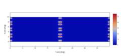
Cheers!
Uh oh!
There was an error while loading.Please reload this page.
Trying toclose#58.
I don't know exactly where do you want to put this functionality, but I open this PR with a working implementation that can be then reorganized as you wish whenever you want.
Basically, I introduced a
compute_dmfunction that from aBrillouinZoneobject with an associated hamiltonian computes the DM. You can provide a custom distribution function to weight the eigenstates as I show below.First, here's a test with a bunch of calculations of a Pt-Au chain with all spin variants at gamma and with 3 k points (files):
Which gives the following maximum differences:
An example of using it to get the LDOS:
Which is basically the same as the LDOS generated by SIESTA selecting the same states:
Cheers!