Repository files navigation

This repository implements Model Predictive Path Integral (MPPI)with approximate dynamics in pytorch. MPPI typically requires actualtrajectory samples, butthis papershowed that it could be done with approximate dynamics (such as with a neural network)using importance sampling.

Thus it can be used in place of other trajectory optimization methodssuch as the Cross Entropy Method (CEM), or random shooting.

New since Aug 2024 smoothing methods, including our own KMPPI, see thesection below on smoothing

pip install pytorch-mppi

for autotuning hyperparameters, install with

pip install pytorch-mppi[tune]

for running tests, install with

pip install pytorch-mppi[test]

for development, clone the repository then install in editable mode

pip install -e.

Seetests/pendulum_approximate.py for usage with a neural network approximatingthe pendulum dynamics. See thenot_batch branch for an easier to readalgorithm. Basic use case is shown below

frompytorch_mppiimportMPPI# create controller with chosen parametersctrl=MPPI(dynamics,running_cost,nx,noise_sigma,num_samples=N_SAMPLES,horizon=TIMESTEPS,lambda_=lambda_,device=d,u_min=torch.tensor(ACTION_LOW,dtype=torch.double,device=d),u_max=torch.tensor(ACTION_HIGH,dtype=torch.double,device=d))# assuming you have a gym-like envobs=env.reset()foriinrange(100):action=ctrl.command(obs)obs,reward,done,_=env.step(action.cpu().numpy())

• pytorch (>= 1.0)
• next state <- dynamics(state, action) function (doesn't have to be true dynamics)
  • state isK x nx,action isK x nu
• cost <- running_cost(state, action) function
  • cost isK x 1, state isK x nx,action isK x nu

• Approximate dynamics MPPI with importance sampling
• Parallel/batch pytorch implementation for accelerated sampling
• Control bounds via sampling control noise from rectified gaussian
• Handle stochastic dynamic models (assuming each call is a sample) by sampling multiple state trajectories for the sameaction trajectory withrollout_samples

terminal_state_cost - function(state (K x T x nx)) -> cost (K x 1) by default there is no terminalcost, but if you experience your trajectory getting close to but never quite reaching the goal, thenhaving a terminal cost can help. The function should scale with the horizon (T) to keep up with thescaling of the running cost.

lambda_ - higher values increases the cost of control noise, so you end up with moresamples around the mean; generally lower values work better (try1e-2)

num_samples - number of trajectories to sample; generally the more the better.Runtime performance scales much better withnum_samples thanhorizon, especiallyif you're using a GPU device (remember to pass that in!)

noise_mu - the default is 0 for all control dimensions, which may work outreally poorly if you have control bounds and the allowed range is not 0-centered.Remember to change this to an appropriate value for non-symmetric control dimensions.

From version 0.8.0 onwards, you can use MPPI variants that smooth the control signal. We've implementedSMPPI as well our own kernel interpolation MPPI (KMPPI). In the base algorithm,you can achieve somewhat smoother trajectories by increasinglambda_; however, that comes at the cost ofoptimality. Explicit smoothing algorithms can achieve smoothness without sacrificing optimality.

We used it and described it in our recent paper (arxiv) and you can cite ituntil we release a work dedicated to KMPPI. Below we show the difference between MPPI, SMPPI, and KMPPI on a toy2D navigation problem where the control is a constrained delta position. You can check it out intests/smooth_mppi.py.

The API is mostly the same, with some additional constructor options:

importpytorch_mppiasmppictrl=mppi.KMPPI(args,kernel=mppi.RBFKernel(sigma=2),# kernel in trajectory time space (1 dimensional)num_support_pts=5,# number of control points to sample, <= horizon**kwargs)

The kernel can be any subclass ofmppi.TimeKernel. It is a kernel in the trajectory time space (1 dimensional).Note that B-spline smoothing can be achieved by using a B-spline kernel. The number of support points is the numberof control points to sample. Any trajectory points in between are interpolated using the kernel. For example if atrajectory horizon is 20 andnum_support_pts is 5, then 5 control points evenly spaced throughout the horizon(with the first and last corresponding to the actual start and end of the trajectory) are sampled. The rest of thetrajectory is interpolated using the kernel. The kernel is applied to the control signal, not the state signal.

MPPI without smoothing

SMPPI smoothing by sampling noise in the action derivative space doesn't work well on this problem

KMPPI smoothing with RBF kernel works well

from version 0.5.0 onwards, you can automatically tune the hyperparameters.A convenient tuner compatible with the popularray tune libraryis implemented. You can select from a variety of cutting edge black-box optimizers such asCMA-ES,HyperOpt,fmfn/BayesianOptimization, and so on.Seetests/auto_tune_parameters.py for an example. A tutorial based on it follows.

The tuner can be used for other controllers as well, but you will need to define the appropriateTunableParameter subclasses.

First we create a toy 2D environment to do controls on and create the controller with somedefault parameters.

importtorchfrompytorch_mppiimportMPPIdevice="cpu"dtype=torch.double# create toy environment to do on control on (default start and goal)env=Toy2DEnvironment(visualize=True,terminal_scale=10)# create MPPI with some initial parametersmppi=MPPI(env.dynamics,env.running_cost,2,terminal_state_cost=env.terminal_cost,noise_sigma=torch.diag(torch.tensor([5.,5.],dtype=dtype,device=device)),num_samples=500,horizon=20,device=device,u_max=torch.tensor([2.,2.],dtype=dtype,device=device),lambda_=1)

We then need to create an evaluation function for the tuner to tune on.It should take no arguments and output aEvaluationResult populated at least by costs.If you don't need rollouts for the cost evaluation, then you can set it to None in the return.Tips for creating the evaluation function are described in comments below:

frompytorch_mppiimportautotune# use the same nominal trajectory to start with for all the evaluations for fairnessnominal_trajectory=mppi.U.clone()# parameters for our sample evaluation function - lots of choices for the evaluation functionevaluate_running_cost=Truenum_refinement_steps=10num_trajectories=5defevaluate():costs= []rollouts= []# we sample multiple trajectories for the same start to goal problem, but in your case you should consider# evaluating over a diverse dataset of trajectoriesforjinrange(num_trajectories):mppi.U=nominal_trajectory.clone()# the nominal trajectory at the start will be different if the horizon's changedmppi.change_horizon(mppi.T)# usually MPPI will have its nominal trajectory warm-started from the previous iteration# for a fair test of tuning we will reset its nominal trajectory to the same random one each time# we manually warm it by refining it for some stepsforkinrange(num_refinement_steps):mppi.command(env.start,shift_nominal_trajectory=False)rollout=mppi.get_rollouts(env.start)this_cost=0rollout=rollout[0]# here we evaluate on the rollout MPPI cost of the resulting trajectories# alternative costs for tuning the parameters are possible, such as just considering terminal costifevaluate_running_cost:fortinrange(len(rollout)-1):this_cost=this_cost+env.running_cost(rollout[t],mppi.U[t])this_cost=this_cost+env.terminal_cost(rollout,mppi.U)rollouts.append(rollout)costs.append(this_cost)# can return None for rollouts if they do not need to be calculatedreturnautotune.EvaluationResult(torch.stack(costs),torch.stack(rollouts))

With this we have enough to start tuning. For example, we can tune iteratively with the CMA-ES optimizer

# these are subclass of TunableParameter (specifically MPPIParameter) that we want to tuneparams_to_tune= [autotune.SigmaParameter(mppi),autotune.HorizonParameter(mppi),autotune.LambdaParameter(mppi)]# create a tuner with a CMA-ES optimizertuner=autotune.Autotune(params_to_tune,evaluate_fn=evaluate,optimizer=autotune.CMAESOpt(sigma=1.0))# tune parameters for a number of iterationsiterations=30foriinrange(iterations):# results of this optimization step are returnedres=tuner.optimize_step()# we can render the rollouts in the environmentenv.draw_rollouts(res.rollouts)# get best results and apply it to the controller# (by default the controller will take on the latest tuned parameter, which may not be best)res=tuner.get_best_result()tuner.apply_parameters(res.param_values)

This is a local search method that optimizes starting from the initially defined parameters.For global searching, we use ray tune compatible searching algorithms. Note that you can modify thesearch space of each parameter, but default reasonable ones are provided.

# can also use a Ray Tune optimizer, see# https://docs.ray.io/en/latest/tune/api_docs/suggestion.html#search-algorithms-tune-search# rather than adapting the current parameters, these optimizers allow you to define a search space for each# and will search on that spacefrompytorch_mppiimportautotune_globalfromray.tune.search.hyperoptimportHyperOptSearchfromray.tune.search.bayesoptimportBayesOptSearch# the global version of the parameters define a reasonable search space for each parameterparams_to_tune= [autotune_global.SigmaGlobalParameter(mppi),autotune_global.HorizonGlobalParameter(mppi),autotune_global.LambdaGlobalParameter(mppi)]# be sure to close any figures before ray tune optimization or they will be duplicatedenv.visualize=Falseplt.close('all')tuner=autotune_global.AutotuneGlobal(params_to_tune,evaluate_fn=evaluate,optimizer=autotune_global.RayOptimizer(HyperOptSearch))# ray tuners cannot be tuned iteratively, but you can specify how many iterations to tune forres=tuner.optimize_all(100)res=tuner.get_best_result()tuner.apply_parameters(res.params)

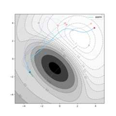
For example tuning hyperparameters (with CMA-ES) only on the toy problem (the nominal trajectory is reset each time so they are sampling from noise):

If you want more than just the best solution found, such as if you want diversityacross hyperparameter values, or if your evaluation function has large uncertainty,then you can directly query past results by

forresintuner.optim.all_res:# the costprint(res.metrics['cost'])# extract the parametersparams=tuner.config_to_params(res.config)print(params)# apply the parameters to the controllertuner.apply_parameters(params)

Alternatively you can try Quality Diversity optimization using theCMA-ME optimizer. This optimizer willtry to optimize for high quality parameters while ensuring there is diversity acrossthem. However, it is very slow and you might be better using aRayOptimizer and selectingfor top results while checking for diversity.To use it, you need to install

pipinstallribs

You then use it as

importpytorch_mppi.autotune_qdoptim=pytorch_mppi.autotune_qd.CMAMEOpt()tuner=autotune_global.AutotuneGlobal(params_to_tune,evaluate_fn=evaluate,optimizer=optim)iterations=10foriinrange(iterations):# results of this optimization step are returnedres=tuner.optimize_step()# we can render the rollouts in the environmentbest_params=optim.get_diverse_top_parameters(5)forresinbest_params:print(res)

Undertests you can find theMPPI method applied to known pendulum dynamicsand approximate pendulum dynamics (with a 2 layer feedforward netestimating the state residual). Using a continuous angle representation(feedingcos(\theta), sin(\theta) instead of\theta directly) makesa huge difference. Although both works, the continuous representationis much more robust to controller parameters and random seed. In addition,the problem of continuing to spin after over-swinging does not appear.

Sample result on approximate dynamics with 100 steps of random policy datato initialize the dynamics:

• pytorch CEM - an alternative MPC shooting method with similar API as thisproject
• pytorch iCEM - alternative sampling based MPC