Repository files navigation

diffeqpy is a package for solving differential equations in Python. It utilizesDifferentialEquations.jl for its core routinesto give high performance solving of many different types of differential equations,including:

• Discrete equations (function maps, discrete stochastic (Gillespie/Markov)simulations)
• Ordinary differential equations (ODEs)
• Split and Partitioned ODEs (Symplectic integrators, IMEX Methods)
• Stochastic ordinary differential equations (SODEs or SDEs)
• Random differential equations (RODEs or RDEs)
• Differential algebraic equations (DAEs)
• Delay differential equations (DDEs)
• Mixed discrete and continuous equations (Hybrid Equations, Jump Diffusions)

directly in Python.

If you have any questions, or just want to chat about solvers/using the package,please feel free to chat in theGitter channel. For bug reports, feature requests, etc., please submit an issue.

To install diffeqpy, use pip:

pip install diffeqpy

and you're good!

• Solving the Lorenz equation faster than SciPy+Numba
• Solving ODEs on GPUs Fast in Python with diffeqpy

Import and setup the solvers available inDifferentialEquations.jl via the command:

fromdiffeqpyimportde

In case only the solvers available inOrdinaryDiffEq.jl are required then use the command:

fromdiffeqpyimportode

The general flow for using the package is to follow exactly as would be donein Julia, except addde. orode. in front. Note thatode. has lesser loading time and a smaller memory footprint compared tode..Most of the commands will work without any modification. Thusthe DifferentialEquations.jl documentationand theDiffEqTutorialsare the main in-depth documentation for this package. Below we will show how totranslate these docs to Python code.

Python does not allow! in function names, so this is alsoa limitation of pyjuliaTo use functions which on the Julia side have a!, likestep!, replace! by_b, for example:

fromdiffeqpyimportdedeff(u,p,t):return-uu0=0.5tspan= (0.,1.)prob=de.ODEProblem(f,u0,tspan)integrator=de.init(prob,de.Tsit5())de.step_b(integrator)

is valid Python code for usingthe integrator interface.

fromdiffeqpyimportdedeff(u,p,t):return-uu0=0.5tspan= (0.,1.)prob=de.ODEProblem(f,u0,tspan)sol=de.solve(prob)

The solution object is the same as the one describedin the DiffEq tutorialsand in thesolution handling documentation(note: the array interface is missing). Thus for example the solution time pointsare saved insol.t and the solution values are saved insol.u. Additionally,the interpolationsol(t) gives a continuous solution.

We can plot the solution values using matplotlib:

importmatplotlib.pyplotaspltplt.plot(sol.t,sol.u)plt.show()

We can utilize the interpolation to get a finer solution:

importnumpyt=numpy.linspace(0,1,100)u=sol(t)plt.plot(t,u)plt.show()

Thecommon interface argumentscan be used to control the solve command. For example, let's usesaveat tosave the solution at everyt=0.1, and let's utilize theVern9() 9th orderRunge-Kutta method along with low tolerancesabstol=reltol=1e-10:

sol=de.solve(prob,de.Vern9(),saveat=0.1,abstol=1e-10,reltol=1e-10)

The set of algorithms for ODEs is describedat the ODE solvers page.

When solving a differential equation, it's pertinent that your derivativefunctionf is fast since it occurs in the inner loop of the solver. We canconvert the entire ode problem to symbolic form, optimize that symbolic form,and emit efficient native code to simulate it usingde.jit to improve theefficiency of the solver at the expense of added setup time:

fast_prob=de.jit(prob)sol=de.solve(fast_prob)

Additionally, you can directly define the functions in Julia. This will alsoallow for specialization and could be helpful to increase the efficiency forrepeat or long calls. This is done viaseval:

jul_f=de.seval("(u,p,t)->-u")# Define the anonymous function in Juliaprob=de.ODEProblem(jul_f,u0,tspan)sol=de.solve(prob)

de.jit, uses ModelingToolkit.jl'smodelingtoolkitize internally and somerestrictions apply. Not all models can be jitted. See themodelingtoolkitize documentationfor more info.

To solve systems of ODEs, simply use an array as your initial condition anddefinef as an array function:

deff(u,p,t):x,y,z=usigma,rho,beta=preturn [sigma* (y-x),x* (rho-z)-y,x*y-beta*z]u0= [1.0,0.0,0.0]tspan= (0.,100.)p= [10.0,28.0,8/3]prob=de.ODEProblem(f,u0,tspan,p)sol=de.solve(prob,saveat=0.01)plt.plot(sol.t,de.transpose(de.stack(sol.u)))plt.show()

or we can draw the phase plot:

us=de.stack(sol.u)frommpl_toolkits.mplot3dimportAxes3Dfig=plt.figure()ax=fig.add_subplot(111,projection='3d')ax.plot(us[0,:],us[1,:],us[2,:])plt.show()

When dealing with systems of equations, in many cases it's helpful to reducememory allocations by using mutating functions. In diffeqpy, the mutatingform adds the mutating vector to the front. Let's make a fast version of theLorenz derivative, i.e. mutating and JIT compiled:

deff(du,u,p,t):x,y,z=usigma,rho,beta=pdu[0]=sigma* (y-x)du[1]=x* (rho-z)-ydu[2]=x*y-beta*zu0= [1.0,0.0,0.0]tspan= (0.,100.)p= [10.0,28.0,2.66]prob=de.ODEProblem(f,u0,tspan,p)jit_prob=de.jit(prob)sol=de.solve(jit_prob)

or using a Julia function:

jul_f=de.seval("""function f(du,u,p,t)  x, y, z = u  sigma, rho, beta = p  du[1] = sigma * (y - x)  du[2] = x * (rho - z) - y  du[3] = x * y - beta * zend""")u0= [1.0,0.0,0.0]tspan= (0.,100.)p= [10.0,28.0,2.66]prob=de.ODEProblem(jul_f,u0,tspan,p)sol=de.solve(prob)

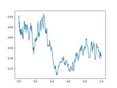
Solving one-dimensonal SDEsdu = f(u,t)dt + g(u,t)dW_t is like an ODE exceptwith an extra function for the diffusion (randomness or noise) term. The stepsfollow theSDE tutorial.

deff(u,p,t):return1.01*udefg(u,p,t):return0.87*uu0=0.5tspan= (0.0,1.0)prob=de.SDEProblem(f,g,u0,tspan)sol=de.solve(prob,reltol=1e-3,abstol=1e-3)plt.plot(sol.t,de.stack(sol.u))plt.show()

An SDE with diagonal noise is where a different Wiener process is applied toevery part of the system. This is common for models with phenomenological noise.Let's add multiplicative noise to the Lorenz equation:

deff(du,u,p,t):x,y,z=usigma,rho,beta=pdu[0]=sigma* (y-x)du[1]=x* (rho-z)-ydu[2]=x*y-beta*zdefg(du,u,p,t):du[0]=0.3*u[0]du[1]=0.3*u[1]du[2]=0.3*u[2]u0= [1.0,0.0,0.0]tspan= (0.,100.)p= [10.0,28.0,2.66]prob=de.jit(de.SDEProblem(f,g,u0,tspan,p))sol=de.solve(prob)# Now let's draw a phase plotus=de.stack(sol.u)frommpl_toolkits.mplot3dimportAxes3Dfig=plt.figure()ax=fig.add_subplot(111,projection='3d')ax.plot(us[0,:],us[1,:],us[2,:])plt.show()

In many cases you may want to share noise terms across the system. This isknown as non-diagonal noise. TheDifferentialEquations.jl SDE Tutorialexplains how the matrix form of the diffusion term corresponds to thesummation style of multiple Wiener processes. Essentially, the row correspondsto which system the term is applied to, and the column is which noise term.Sodu[i,j] is the amount of noise due to thejth Wiener process that'sapplied tou[i]. We solve the Lorenz system with correlated noise as follows:

deff(du,u,p,t):x,y,z=usigma,rho,beta=pdu[0]=sigma* (y-x)du[1]=x* (rho-z)-ydu[2]=x*y-beta*zdefg(du,u,p,t):du[0,0]=0.3*u[0]du[1,0]=0.6*u[0]du[2,0]=0.2*u[0]du[0,1]=1.2*u[1]du[1,1]=0.2*u[1]du[2,1]=0.3*u[1]u0= [1.0,0.0,0.0]tspan= (0.0,100.0)p= [10.0,28.0,2.66]nrp=numpy.zeros((3,2))prob=de.SDEProblem(f,g,u0,tspan,p,noise_rate_prototype=nrp)jit_prob=de.jit(prob)sol=de.solve(jit_prob,saveat=0.005)# Now let's draw a phase plotus=de.stack(sol.u)frommpl_toolkits.mplot3dimportAxes3Dfig=plt.figure()ax=fig.add_subplot(111,projection='3d')ax.plot(us[0,:],us[1,:],us[2,:])plt.show()

Here you can see that the warping effect of the noise correlations is quite visible!

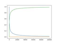
A differential-algebraic equation is defined by an implicit functionf(du,u,p,t)=0. All of the controls are the same as the other examples, excepthere you define a function which returns the residuals for each part of theequation to define the DAE. The initial valueu0 and the initial derivativedu0 are required, though they do not necessarily have to satisfyf (knownas inconsistent initial conditions). The methods will automatically findconsistent initial conditions. In order for this to occur,differential_varsmust be set. This vector states which of the variables are differential (have aderivative term), withfalse meaning that the variable is purely algebraic.

This example shows how to solve the Robertson equation:

deff(du,u,p,t):resid1=-0.04*u[0]+1e4*u[1]*u[2]-du[0]resid2=+0.04*u[0]-3e7*u[1]**2-1e4*u[1]*u[2]-du[1]resid3=u[0]+u[1]+u[2]-1.0return [resid1,resid2,resid3]u0= [1.0,0.0,0.0]du0= [-0.04,0.04,0.0]tspan= (0.0,100000.0)differential_vars= [True,True,False]prob=de.DAEProblem(f,du0,u0,tspan,differential_vars=differential_vars)sol=de.solve(prob)

and the in-place JIT compiled form:

deff(resid,du,u,p,t):resid[0]=-0.04*u[0]+1e4*u[1]*u[2]-du[0]resid[1]=+0.04*u[0]-3e7*u[1]**2-1e4*u[1]*u[2]-du[1]resid[2]=u[0]+u[1]+u[2]-1.0prob=de.DAEProblem(f,du0,u0,tspan,differential_vars=differential_vars)jit_prob=de.jit(prob)# Error: no method matching matching modelingtoolkitize(::SciMLBase.DAEProblem{...})sol=de.solve(jit_prob)

Mass matrix DAEs, along with many other forms, can be handled by doing an explicit conversion to the Julia types.Seethe PythonCall module's documentation for more details.

As an example, let's convertthe mass matrix ODE tutorial in diffeqpy.To do this, the one aspect we need to handle is the conversion of the mass matrix in to a Julia array object. This is done as follows:

fromdiffeqpyimportdefromjuliacallimportMainasjlimportnumpyasnpdefrober(du,u,p,t):y1,y2,y3=uk1,k2,k3=pdu[0]=-k1*y1+k3*y2*y3du[1]=k1*y1-k3*y2*y3-k2*y2**2du[2]=y1+y2+y3-1returnM=np.array([[1.0,0.0,0.0],[0.0,1.0,0.0],[0.0,0.0,0.0]])f=de.ODEFunction(rober,mass_matrix=jl.convert(jl.Array,M))prob_mm=de.ODEProblem(f, [1.0,0.0,0.0], (0.0,1e5), (0.04,3e7,1e4))sol=de.solve(prob_mm,de.Rodas5P(),reltol=1e-8,abstol=1e-8)

Notice the only addition is to create thenp.array object and to perform the manual conversion viajl.convert(jl.Array,M) to receive theJuliaArray object. This can be done in any case where diffeqpy is not adequately auto-converting to the right Julia type. In some cases thiscan be used to improve performance, though here we do it simply for compatability.

Similarly, sparse matrices can be passed in much the same way. For example:

importscipyspM=scipy.sparse.csr_array(M)jl.seval("using SparseArrays")f=de.ODEFunction(rober,mass_matrix=jl.convert(jl.SparseMatrixCSC,M))prob_mm=de.ODEProblem(f, [1.0,0.0,0.0], (0.0,1e5), (0.04,3e7,1e4))sol=de.solve(prob_mm,de.Rodas5P(),reltol=1e-8,abstol=1e-8)

A delay differential equation is an ODE which allows the use of previous values.In this case, the function needs to be a JIT compiled Julia function. It looksjust like the ODE, except in this case there is a functionh(p,t) which allowsyou to interpolate and grab previous values.

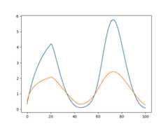
We must provide a history functionh(p,t) that gives values foru beforet0.Here we assume that the solution was constant before the initial time point.Additionally, we passconstant_lags = [20.0] to tell the solver that onlyconstant-time lags were used and what the lag length was. This helps improvethe solver accuracy by accurately stepping at the points of discontinuity.Together this is:

f=de.seval("""function f(du, u, h, p, t)  du[1] = 1.1/(1 + sqrt(10)*(h(p, t-20)[1])^(5/4)) - 10*u[1]/(1 + 40*u[2])  du[2] = 100*u[1]/(1 + 40*u[2]) - 2.43*u[2]end""")u0= [1.05767027/3,1.030713491/3]h=de.seval("""function h(p,t)  [1.05767027/3, 1.030713491/3]end""")tspan= (0.0,100.0)constant_lags= [20.0]prob=de.DDEProblem(f,u0,h,tspan,constant_lags=constant_lags)sol=de.solve(prob,saveat=0.1)u1= [sol.u[i][0]foriinrange(0,len(sol.u))]u2= [sol.u[i][1]foriinrange(0,len(sol.u))]importmatplotlib.pyplotaspltplt.plot(sol.t,u1)plt.plot(sol.t,u2)plt.show()

Notice that the solver accurately is able to simulate the kink (discontinuity)att=20 due to the discontinuity of the derivative at the initial time point!This is why declaring discontinuities can enhance the solver accuracy.

In many cases one is interested in solving the same ODE many times over manydifferent initial conditions and parameters. In diffeqpy parlance this is calledan ensemble solve. diffeqpy inherits the parallelism tools of theSciML ecosystem that are used for things likeautomated equation discovery and acceleration.Here we will demonstrate using these parallel tools to accelerate the solvingof an ensemble.

First, let's define the JIT-accelerated Lorenz equation like before:

fromdiffeqpyimportdedeff(u,p,t):x,y,z=usigma,rho,beta=preturn [sigma* (y-x),x* (rho-z)-y,x*y-beta*z]u0= [1.0,0.0,0.0]tspan= (0.,100.)p= [10.0,28.0,8/3]prob=de.ODEProblem(f,u0,tspan,p)fast_prob=de.jit32(prob)sol=de.solve(fast_prob,saveat=0.01)

Note that here we usedde.jit32 to JIT-compile the problem into aFloat32 form in order to make it moreefficient on most GPUs.

Now we use theEnsembleProblem as defined on theensemble parallelism page of the documentation:Let's build an ensemble by utilizing uniform random numbers to randomize theinitial conditions and parameters:

importrandomdefprob_func(prob,i,rep):returnde.remake(prob,u0=[random.uniform(0,1)*u0[i]foriinrange(0,3)],p=[random.uniform(0,1)*p[i]foriinrange(0,3)])ensembleprob=de.EnsembleProblem(fast_prob,prob_func=prob_func,safetycopy=False)

Now we solve the ensemble in serial:

sol=de.solve(ensembleprob,de.Tsit5(),de.EnsembleSerial(),trajectories=10000,saveat=0.01)

To add GPUs to the mix, we need to bring inDiffEqGPU.The commandfrom diffeqpy import cuda will install CUDA for you and bring all of the bindings into the returned object:

Now we simply useEnsembleGPUKernel(cuda.CUDABackend()) with aGPU-specialized ODE solvercuda.GPUTsit5() to solve 10,000 ODEs on the GPU inparallel:

sol=de.solve(ensembleprob,cuda.GPUTsit5(),cuda.EnsembleGPUKernel(cuda.CUDABackend()),trajectories=10000,saveat=0.01)

For the full list of choices for specialized GPU solvers, seethe DiffEqGPU.jl documentation.

Note thatEnsembleGPUArray can be used as well, like:

sol=de.solve(ensembleprob,de.Tsit5(),cuda.EnsembleGPUArray(cuda.CUDABackend()),trajectories=10000,saveat=0.01)

though we highly recommend theEnsembleGPUKernel methods for more speed. Giventhe way the JIT compilation performed will also ensure that the faster kernelgeneration methods work,EnsembleGPUKernel is almost certainly thebetter choice in most applications.

To see how much of an effect the parallelism has, let's test this against R'sdeSolve package. This is exactly the same problem as the documentation examplefor deSolve, so let's copy that verbatim and then add a function to do theensemble generation:

importnumpyasnpfromscipy.integrateimportodeintdeflorenz(state,t,sigma,beta,rho):x,y,z=statedx=sigma* (y-x)dy=x* (rho-z)-ydz=x*y-beta*zreturn [dx,dy,dz]sigma=10.0beta=8.0/3.0rho=28.0p= (sigma,beta,rho)y0= [1.0,1.0,1.0]t=np.arange(0.0,100.0,0.01)result=odeint(lorenz,y0,t,p)

Usinglapply to generate the ensemble we get:

importtimeitdeftime_func():foritrinrange(1,1001):result=odeint(lorenz,y0,t,p)timeit.Timer(time_func).timeit(number=1)# 38.08861699999761 seconds

Now let's see how the JIT-accelerated serial Julia version stacks up against that:

deftime_func():sol=de.solve(ensembleprob,de.Tsit5(),de.EnsembleSerial(),trajectories=1000,saveat=0.01)timeit.Timer(time_func).timeit(number=1)# 3.1903300999983912

Julia is already about 12x faster than the pure Python solvers here! Now let's addGPU-acceleration to the mix:

deftime_func():sol=de.solve(ensembleprob,cuda.GPUTsit5(),cuda.EnsembleGPUKernel(cuda.CUDABackend()),trajectories=1000,saveat=0.01)timeit.Timer(time_func).timeit(number=1)# 0.013322799997695256

Already 2900x faster than SciPy! But the GPU acceleration is made for massivelyparallel problems, so let's up the trajectories a bit. We will not use moretrajectories from R because that would take too much computing power, so let'ssee what happens to the Julia serial and GPU at 10,000 trajectories:

deftime_func():sol=de.solve(ensembleprob,de.Tsit5(),de.EnsembleSerial(),trajectories=10000,saveat=0.01)timeit.Timer(time_func).timeit(number=1)# 68.80795999999827

deftime_func():sol=de.solve(ensembleprob,cuda.GPUTsit5(),cuda.EnsembleGPUKernel(cuda.CUDABackend()),trajectories=10000,saveat=0.01)timeit.Timer(time_func).timeit(number=1)# 0.10774460000175168

To compare this to the pure Julia code:

using OrdinaryDiffEq, DiffEqGPU, CUDA, StaticArraysfunctionlorenz(u, p, t)    σ= p[1]    ρ= p[2]    β= p[3]    du1= σ* (u[2]- u[1])    du2= u[1]* (ρ- u[3])- u[2]    du3= u[1]* u[2]- β* u[3]returnSVector{3}(du1, du2, du3)endu0= SA[1.0f0;0.0f0;0.0f0]tspan= (0.0f0,10.0f0)p= SA[10.0f0,28.0f0,8/3.0f0]prob=ODEProblem{false}(lorenz, u0, tspan, p)prob_func= (prob, i, repeat)->remake(prob, p= (@SVectorrand(Float32,3)).* p)monteprob=EnsembleProblem(prob, prob_func= prob_func, safetycopy=false)@time sol=solve(monteprob,GPUTsit5(),EnsembleGPUKernel(CUDA.CUDABackend()),    trajectories=10_000,    saveat=0.01);# 0.014481 seconds (257.64 k allocations: 13.130 MiB)

which is about an order of magnitude faster for computing 10,000 trajectories,note that the major factors are that we cannot define 32-bit floating point valuesfrom Python and theprob_func for generating the initial conditions and parametersis a major bottleneck since this function is written in Python.

To see how this scales in Julia, let's take it to insane heights. First, let'sreduce the amount we're saving:

@time sol=solve(monteprob,GPUTsit5(),EnsembleGPUKernel(CUDA.CUDABackend()),trajectories=10_000,saveat=1.0f0)0.015040 seconds (257.64 k allocations:13.130 MiB)

This highlights that controlling memory pressure is key with GPU usage: you willget much better performance when requiring less saved points on the GPU.

@time sol=solve(monteprob,GPUTsit5(),EnsembleGPUKernel(CUDA.CUDABackend()),trajectories=100_000,saveat=1.0f0)# 0.150901 seconds (2.60 M allocations: 131.576 MiB)

compared to serial:

@time sol=solve(monteprob,Tsit5(),EnsembleSerial(),trajectories=100_000,saveat=1.0f0)# 22.136743 seconds (16.40 M allocations: 1.628 GiB, 42.98% gc time)

And now we start to see that scaling power! Let's solve 1 million trajectories:

@time sol=solve(monteprob,GPUTsit5(),EnsembleGPUKernel(CUDA.CUDABackend()),trajectories=1_000_000,saveat=1.0f0)# 1.031295 seconds (3.40 M allocations: 241.075 MiB)

For reference, let's look at deSolve with the change to only save that much:

t=np.arange(0.0,100.0,1.0)deftime_func():foritrinrange(1,1001):result=odeint(lorenz,y0,t,p)timeit.Timer(time_func).timeit(number=1)# 37.42609280000033

The GPU version is solving 1000x as many trajectories, 37x as fast! So conclusion,if you need the most speed, you may want to move to the Julia version to get themost out of your GPU due to Float32's, and when using GPUs make sure it's a problemwith a relatively average or low memory pressure, and these methods will giveorders of magnitude acceleration compared to what you might be used to.

Just like DiffEqGPU.jl, diffeqpy supports many different GPU venders.from diffeqpy import cudais just for cuda, but the following others are supported:

• from diffeqpy import cuda withcuda.CUDABackend for NVIDIA GPUs via CUDA
• from diffeqpy import amdgpu withamdgpu.AMDGPUBackend for AMD GPUs
• from diffeqpy import oneapi withoneapi.oneAPIBackend for Intel's oneAPI GPUs
• from diffeqpy import metal withmetal.MetalBackend for Apple's Metal GPUs (on M-series processors)

For more information, seethe DiffEqGPU.jl documentation.

• Autodiff does not work on Python functions. When applicable, either define the derivative functionas a Julia function or set the algorithm to use finite differencing, i.e.Rodas5(autodiff=false).All default methods use autodiff.
• Delay differential equations have to use Julia-defined functions otherwise the history function isnot appropriately typed with the overloads.

Unit tests can be run bytox.

tox

In case you encounter silent failure fromtox, try running it with-- -s (e.g.,tox -e py36 -- -s) where-s option (--capture=no,i.e., don't capture stdio) is passed topy.test. It may show anerror message"error initializing LibGit2 module". In this case,setting environment variableSSL_CERT_FILE may help; e.g., try:

SSL_CERT_FILE=PATH/TO/cert.pem tox -e py36

See also:julia#18693.