


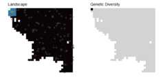
Generate continuous maps of genetic diversity using moving windowswith options for rarefaction, interpolation, and masking.
Please cite the original Bishop et al. (2023) paper if you use thispackage:
Bishop, A. P., Chambers, E. A., & Wang, I. J. (2023).Generating continuous maps of genetic diversity using moving windows.Methods in Ecology and Evolution, 14,1175–1181.http://doi.org/10.1111/2041-210X.14090
Checkout ourMethodsblog post about wingen for a quick overview of the package and itsuses.
Install the released version of wingen from CRAN:
install.packages("wingen")Or install the development version from GitHub:
# install.packages("devtools")devtools::install_github("AnushaPB/wingen")The following example demonstrates the basic functionality of wingenusing asmall subset (100 variant loci x 100 samples) of thesimulated data fromBishop etal. (2023).
library(wingen)# Load ggplot for plottinglibrary(ggplot2)# Load example dataload_middle_earth_ex()The core function of this package iswindow_gd(), whichtakes as inputs a vcfR object (or a path to a .vcf file), samplecoordinates (as a data.frame, matrix, or sf object), and a raster layer(as a SpatRaster or RasterLayer) which the moving window will slideacross. Users can control the genetic diversity statistic that iscalculated (stat), the window dimensions(wdim), the aggregation factor to use on the raster(fact), whether to perform rarefaction(rarify), and other aspects of the moving windowcalculations. Additional arguments for this function are described inthe vignette and function documentation.
# Run moving window calculations of pi with rarefactionwgd<-window_gd(lotr_vcf, lotr_coords, lotr_lyr,stat ="pi",wdim =7,fact =3,rarify =TRUE)# Use ggplot_gd() to plot the genetic diversity layer and ggplot_count() to plot the sample counts layerggplot_gd(wgd)+ggtitle("Moving window pi")
ggplot_count(wgd)+ggtitle("Moving window sample counts")
Next, the output fromwindow_gd() can be interpolatedusing kriging with thewkrig_gd() function.
# Interpolate to a higher resolutionkrige_layer<-disagg(wgd,2)kgd<-wkrig_gd(wgd, krige_layer)Finally, the output fromwkrig_gd() (orwindow_gd()) can be masked to exclude areas that falloutside of the study area or that were undersampled.
# Mask results that fall outside of the "range"mgd<-mask_gd(kgd, lotr_range)# Plot resultsggplot_gd(kgd)+ggtitle("Kriged pi")
ggplot_gd(mgd)+ggtitle("Masked pi")
For an extended walk through, see the package vignette:
vignette("wingen-vignette")A pdf of the vignette can also be foundhere
Example analyses fromBishop et al. (2023)can be found in thepaperexdirectory.