


deeptime extends the functionality of other plottingpackages (notably{ggplot2}) to help facilitate theplotting of data over long time intervals, including, but not limitedto, geological, evolutionary, and ecological data. The primary goal ofdeeptime is to enable users to add highly customizabletimescales to their visualizations. Other functions are also included toassist with other areas of deep time visualization.
# get the stable version from CRANinstall.packages("deeptime")# or get the development version from github# install.packages("devtools")devtools::install_github("willgearty/deeptime")library(deeptime)library(ggplot2)library(dplyr)The main function ofdeeptime iscoord_geo(), which functions just likecoord_trans() from{ggplot2}. You can use thisfunction to add highly customizable timescales to a wide variety ofggplots.
library(divDyn)data(corals)# this is not a proper diversity curve but it gets the point acrosscoral_div<- corals%>%filter(stage!="")%>%group_by(stage)%>%summarise(n =n())%>%mutate(stage_age = (stages$max_age[match(stage, stages$name)]+ stages$min_age[match(stage, stages$name)])/2)ggplot(coral_div)+geom_line(aes(x = stage_age,y = n))+scale_x_reverse("Age (Ma)")+ylab("Coral Genera")+coord_geo(xlim =c(250,0),ylim =c(0,1700))+theme_classic(base_size =16)
# Load packageslibrary(gsloid)# Plot two different timescalesggplot(lisiecki2005)+geom_line(aes(x = d18O,y = Time/1000),orientation ="y")+scale_y_reverse("Time (Ma)")+scale_x_reverse("\u03B418O")+coord_geo(dat =list("Geomagnetic Polarity Chron","Planktic foraminiferal Primary Biozones"),xlim =c(6,2),ylim =c(5.5,0),pos =list("l","r"),rot =90,skip ="PL4",size =list(5,4) )+theme_classic(base_size =16)
# Load packageslibrary(ggtree)library(rphylopic)# Get vertebrate phylogenylibrary(phytools)data(vertebrate.tree)vertebrate.tree$tip.label[vertebrate.tree$tip.label=="Myotis_lucifugus"]<-"Vespertilioninae"vertebrate_data<-data.frame(species = vertebrate.tree$tip.label,name = vertebrate.tree$tip.label)# Plot the phylogeny with a timescalerevts(ggtree(vertebrate.tree,size =1))%<+% vertebrate_data+geom_phylopic(aes(name = name),size =25)+scale_x_continuous("Time (Ma)",breaks =seq(-500,0,100),labels =seq(500,0,-100),limits =c(-500,0),expand =expansion(mult =0))+scale_y_continuous(guide =NULL)+coord_geo_radial(dat ="periods",end =0.5* pi)+theme_classic(base_size =16)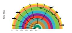
library(palaeoverse)# Filter occurrencesoccdf<-subset(tetrapods, accepted_rank=="genus")occdf<-subset(occdf, accepted_name%in%c("Eryops","Dimetrodon","Diadectes","Diictodon","Ophiacodon","Diplocaulus","Benthosuchus"))# Plot occurrencesggplot(data = occdf)+geom_points_range(aes(x = (max_ma+ min_ma)/2,y = accepted_name))+scale_x_reverse(name ="Time (Ma)")+ylab(NULL)+coord_geo(pos =list("bottom","bottom"),dat =list("stages","periods"),abbrv =list(TRUE,FALSE),expand =TRUE,size ="auto")+theme_classic(base_size =16)
# Load packageslibrary(rmacrostrat)library(ggrepel)# Retrieve the Macrostrat units in the San Juan Basin columnsan_juan_units<-get_units(column_id =489,interval_name ="Cretaceous")# Specify x_min and x_max in dataframesan_juan_units$x_min<-0san_juan_units$x_max<-1# Tweak values for overlapping unitssan_juan_units$x_max[10]<-0.5san_juan_units$x_min[11]<-0.5# Add midpoint age for plottingsan_juan_units$m_age<- (san_juan_units$b_age+ san_juan_units$t_age)/2# Get lithology definitionsliths<-def_lithologies()# Get the primary lithology for each unitsan_juan_units$lith_prim<-sapply(san_juan_units$lith,function(df) { df$name[which.max(df$prop)]})# Get the pattern codes for those lithologiessan_juan_units$pattern<-factor(liths$fill[match(san_juan_units$lith_prim, liths$name)])# Plot with pattern fillsggplot(san_juan_units,aes(ymin = b_age,ymax = t_age,xmin = x_min,xmax = x_max))+# Plot units, patterned by rock typegeom_rect(aes(fill = pattern),color ="black")+scale_fill_geopattern(name =NULL,breaks =factor(liths$fill),labels = liths$name)+# Add text labelsgeom_text_repel(aes(x = x_max,y = m_age,label = unit_name),size =3.5,hjust =0,force =2,min.segment.length =0,direction ="y",nudge_x =rep_len(x =c(2,3),length.out =17))+# Add geological time scalecoord_geo(pos ="left",dat =list("stages"),rot =90)+# Reverse direction of y-axisscale_y_reverse(limits =c(145,66),n.breaks =10,name ="Time (Ma)")+# Remove x-axis guide and titlescale_x_continuous(NULL,guide =NULL)+# Choose theme and font sizetheme_classic(base_size =14)+# Make tick labels blacktheme(legend.position ="bottom",legend.key.size =unit(1,'cm'),axis.text.y =element_text(color ="black"))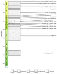
If you use the deeptime R package in your work, please cite as:
Gearty, W. 2025. deeptime: an R package that facilitates highlycustomizable and reproducible visualizations of data over geologicaltime intervals.Big Earth Data. doi:10.1080/20964471.2025.2537516.