


An R package with a set of functions to calibrate time-specificecological niche models. Time-specific niche modeling (TENM) is a novelapproach that allows calibrating niche models with high temporalresolution spatial information, which aims to reduce niche estimationbiases. Although TENM could improve distribution estimates, few workshave used them. The goal oftenm R package is to providemethods and functions to calibrate time-specific niche models, lettingusers execute a strict calibration and selection process of niche modelsbased on ellipsoids, as well as functions to project the potentialdistribution in the present and in global change scenarios.
You can install the development version of tenm fromGitHub with:
if (!require('devtools'))install.packages('devtools')devtools::install_github("luismurao/tenm")# If you want to build vignette, install pandoc before and thendevtools::install_github('luismurao/tenm',build_vignettes=TRUE)We start with a simple example to show the basic functions of thepackage. We will work with a dataset ofAbroniagraminea, an endemic lizard from the Mexican Sierra MadreOriental.
First, we load thetenm R package.
library(tenm)## basic example codeNow we load theabronia dataset, which containsgeographical information about the presence ofAbronia gramineain its area of distribution. This dataset has also information about theyear of observation and theGBIFdoi.
data("abronia")head(abronia)#> species decimalLongitude decimalLatitude year#> 1 Abronia graminea -98.17773 19.96523 2014#> 2 Abronia graminea -98.13753 19.87006 2014#> 3 Abronia graminea -98.07042 19.89668 2014#> 4 Abronia graminea -98.13003 19.86861 2014#> 5 Abronia graminea -98.14894 19.84450 2014#> 6 Abronia graminea -98.15909 19.86878 2014#> gbif_doi#> 1 https://doi.org/10.15468/dl.teyjm9#> 2 https://doi.org/10.15468/dl.teyjm9#> 3 https://doi.org/10.15468/dl.teyjm9#> 4 https://doi.org/10.15468/dl.teyjm9#> 5 https://doi.org/10.15468/dl.teyjm9#> 6 https://doi.org/10.15468/dl.teyjm9dim(abronia)#> [1] 106 5We plot the geographic information to see howAbroniagraminea is distributed.
colorss<-hcl.colors(length(unique(abronia$year)))par(mar=c(4,4,2,2))plot(abronia$decimalLongitude, abronia$decimalLatitude,col=colorss,pch=19,cex=0.75,xlab="Longitude",ylab="Latitude",xlim=c(-98.35,-96.7))legend("bottomleft",legend =sort(unique(abronia$year))[1:20],cex=0.85,pt.cex =1,bty ="n",pch=19,col =colorss[1:20])legend("bottomright",legend =sort(unique(abronia$year))[21:length(unique(abronia$year))],cex=0.85,pt.cex =1,bty ="n",pch=19,col =colorss[21:length(unique(abronia$year))])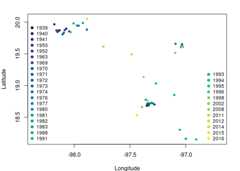
Fig. 1. Occurrence points ofAbronia graminea. Colors representthe year of observation.
Note that some occurrences are overlapped but belong todifferent years.
A relevant step when curating occurrence data is to eliminateduplicated geographical information, which depends on several factors,including spatial autocorrelation and the spatial resolution of themodeling layers. Let’s see what happens when we eliminate duplicatedinformation as defined by the spatial resolution of our modeling layers.To do this, we will use thetenm::clean_dup function of thetenm R package.
# Load a modeling layertempora_layers_dir<-system.file("extdata/bio",package ="tenm")tenm_mask<- terra::rast(file.path(tempora_layers_dir,"1939/bio_01.tif"))ab_1<- tenm::clean_dup(data =abronia,longitude ="decimalLongitude",latitude ="decimalLatitude",threshold = terra::res(tenm_mask),by_mask =FALSE,raster_mask =NULL)tidyr::as_tibble(ab_1)#> # A tibble: 10 × 5#> species decimalLongitude decimalLatitude year gbif_doi#> <chr> <dbl> <dbl> <int> <chr>#> 1 Abronia graminea -97.5 19.5 1995 https://doi.org/10.1…#> 2 Abronia graminea -97.0 18.2 1993 https://doi.org/10.1…#> 3 Abronia graminea -98.0 19.8 1980 https://doi.org/10.1…#> 4 Abronia graminea -97.7 19.6 2012 https://doi.org/10.1…#> 5 Abronia graminea -97.9 20.1 2015 https://doi.org/10.1…#> 6 Abronia graminea -97.4 18.5 1952 https://doi.org/10.1…#> 7 Abronia graminea -97.1 18.9 1998 https://doi.org/10.1…#> 8 Abronia graminea -97.3 19.0 1983 https://doi.org/10.1…#> 9 Abronia graminea -97.3 18.7 1973 https://doi.org/10.1…#> 10 Abronia graminea -97.0 19.7 1972 https://doi.org/10.1…After applying our spatial thinning, we obtained only tenobservations from 106 occurrences. We lost a lot of information!!! Thefunctiontenm::clean_dup has a method to clean duplicatedrecords according to a raster mask layer. The above avoids losingrecords that might occur in different pixels but fall within thedistance used as threshold for cleaning.
ab_by_mask<- tenm::clean_dup(data =abronia,longitude ="decimalLongitude",latitude ="decimalLatitude",threshold = terra::res(tenm_mask),by_mask =TRUE,raster_mask = tenm_mask)tidyr::as_tibble(ab_by_mask)#> # A tibble: 16 × 5#> species decimalLongitude decimalLatitude year gbif_doi#> <chr> <dbl> <dbl> <int> <chr>#> 1 Abronia graminea -98.2 20.0 2014 https://doi.org/10.1…#> 2 Abronia graminea -98.1 19.9 2014 https://doi.org/10.1…#> 3 Abronia graminea -98.1 19.8 2014 https://doi.org/10.1…#> 4 Abronia graminea -97.9 19.9 2014 https://doi.org/10.1…#> 5 Abronia graminea -97.3 18.7 1963 https://doi.org/10.1…#> 6 Abronia graminea -97.1 18.3 1996 https://doi.org/10.1…#> 7 Abronia graminea -97.4 18.8 1941 https://doi.org/10.1…#> 8 Abronia graminea -97.4 18.7 1988 https://doi.org/10.1…#> 9 Abronia graminea -97.0 19.6 1991 https://doi.org/10.1…#> 10 Abronia graminea -97.4 19.1 2002 https://doi.org/10.1…#> 11 Abronia graminea -97.5 19.5 1995 https://doi.org/10.1…#> 12 Abronia graminea -97.0 18.2 1993 https://doi.org/10.1…#> 13 Abronia graminea -97.7 19.6 2012 https://doi.org/10.1…#> 14 Abronia graminea -97.9 20.1 2015 https://doi.org/10.1…#> 15 Abronia graminea -97.1 18.9 1998 https://doi.org/10.1…#> 16 Abronia graminea -97.3 19.0 1983 https://doi.org/10.1…We recovered 6 records, not bad! On the other hand, we did notaccount for the fact that some occurrences come from different years.Thetenm package is designed to deal with occurrencescoming from different periods as long as the user has environmentallayers matching the years of occurrence observations.
Let’s apply the functions and methods to work with time-specificniche models. First, we load our data.
library(tenm)data("abronia")Now, we indicate the path where our time-specific modeling layers arelocated.
tempora_layers_dir<-system.file("extdata/bio",package ="tenm")print(tempora_layers_dir)#> [1] "/home/luis/R/x86_64-pc-linux-gnu-library/4.4/tenm/extdata/bio"We explore the structure of the directory that contains our modelinglayers.
list.dirs(tempora_layers_dir,recursive =FALSE)#> [1] "/home/luis/R/x86_64-pc-linux-gnu-library/4.4/tenm/extdata/bio/1939"#> [2] "/home/luis/R/x86_64-pc-linux-gnu-library/4.4/tenm/extdata/bio/1940"#> [3] "/home/luis/R/x86_64-pc-linux-gnu-library/4.4/tenm/extdata/bio/1941"#> [4] "/home/luis/R/x86_64-pc-linux-gnu-library/4.4/tenm/extdata/bio/1950"#> [5] "/home/luis/R/x86_64-pc-linux-gnu-library/4.4/tenm/extdata/bio/1952"#> [6] "/home/luis/R/x86_64-pc-linux-gnu-library/4.4/tenm/extdata/bio/1963"#> [7] "/home/luis/R/x86_64-pc-linux-gnu-library/4.4/tenm/extdata/bio/1969"#> [8] "/home/luis/R/x86_64-pc-linux-gnu-library/4.4/tenm/extdata/bio/1970"#> [9] "/home/luis/R/x86_64-pc-linux-gnu-library/4.4/tenm/extdata/bio/1971"#> [10] "/home/luis/R/x86_64-pc-linux-gnu-library/4.4/tenm/extdata/bio/1972"#> [11] "/home/luis/R/x86_64-pc-linux-gnu-library/4.4/tenm/extdata/bio/1973"#> [12] "/home/luis/R/x86_64-pc-linux-gnu-library/4.4/tenm/extdata/bio/1974"#> [13] "/home/luis/R/x86_64-pc-linux-gnu-library/4.4/tenm/extdata/bio/1976"#> [14] "/home/luis/R/x86_64-pc-linux-gnu-library/4.4/tenm/extdata/bio/1977"#> [15] "/home/luis/R/x86_64-pc-linux-gnu-library/4.4/tenm/extdata/bio/1980"#> [16] "/home/luis/R/x86_64-pc-linux-gnu-library/4.4/tenm/extdata/bio/1981"#> [17] "/home/luis/R/x86_64-pc-linux-gnu-library/4.4/tenm/extdata/bio/1982"#> [18] "/home/luis/R/x86_64-pc-linux-gnu-library/4.4/tenm/extdata/bio/1983"#> [19] "/home/luis/R/x86_64-pc-linux-gnu-library/4.4/tenm/extdata/bio/1988"#> [20] "/home/luis/R/x86_64-pc-linux-gnu-library/4.4/tenm/extdata/bio/1991"#> [21] "/home/luis/R/x86_64-pc-linux-gnu-library/4.4/tenm/extdata/bio/1993"#> [22] "/home/luis/R/x86_64-pc-linux-gnu-library/4.4/tenm/extdata/bio/1994"#> [23] "/home/luis/R/x86_64-pc-linux-gnu-library/4.4/tenm/extdata/bio/1995"#> [24] "/home/luis/R/x86_64-pc-linux-gnu-library/4.4/tenm/extdata/bio/1996"#> [25] "/home/luis/R/x86_64-pc-linux-gnu-library/4.4/tenm/extdata/bio/1998"#> [26] "/home/luis/R/x86_64-pc-linux-gnu-library/4.4/tenm/extdata/bio/2002"#> [27] "/home/luis/R/x86_64-pc-linux-gnu-library/4.4/tenm/extdata/bio/2008"#> [28] "/home/luis/R/x86_64-pc-linux-gnu-library/4.4/tenm/extdata/bio/2011"#> [29] "/home/luis/R/x86_64-pc-linux-gnu-library/4.4/tenm/extdata/bio/2012"#> [30] "/home/luis/R/x86_64-pc-linux-gnu-library/4.4/tenm/extdata/bio/2014"#> [31] "/home/luis/R/x86_64-pc-linux-gnu-library/4.4/tenm/extdata/bio/2015"#> [32] "/home/luis/R/x86_64-pc-linux-gnu-library/4.4/tenm/extdata/bio/2016"Note that the directory contains other directories named withthe dates of the modeling layers. Now, we explore some of thesedated directories.
# Directory for year 1939list.files(list.dirs(tempora_layers_dir,recursive =FALSE)[1],pattern =".tif$")#> [1] "bio_01.tif" "bio_02.tif" "bio_03.tif" "bio_04.tif" "bio_05.tif"#> [6] "bio_06.tif" "bio_07.tif" "bio_08.tif" "bio_09.tif" "bio_10.tif"#> [11] "bio_11.tif" "bio_12.tif" "bio_13.tif" "bio_14.tif" "bio_15.tif"#> [16] "bio_16.tif" "bio_17.tif" "bio_18.tif" "bio_19.tif"# Directory for year 1972list.files(list.dirs(tempora_layers_dir,recursive =FALSE)[10],pattern =".tif$")#> [1] "bio_01.tif" "bio_02.tif" "bio_03.tif" "bio_04.tif" "bio_05.tif"#> [6] "bio_06.tif" "bio_07.tif" "bio_08.tif" "bio_09.tif" "bio_10.tif"#> [11] "bio_11.tif" "bio_12.tif" "bio_13.tif" "bio_14.tif" "bio_15.tif"#> [16] "bio_16.tif" "bio_17.tif" "bio_18.tif" "bio_19.tif"# Directory for year 2014list.files(list.dirs(tempora_layers_dir,recursive =FALSE)[30],pattern =".tif$")#> [1] "bio_01.tif" "bio_02.tif" "bio_03.tif" "bio_04.tif" "bio_05.tif"#> [6] "bio_06.tif" "bio_07.tif" "bio_08.tif" "bio_09.tif" "bio_10.tif"#> [11] "bio_11.tif" "bio_12.tif" "bio_13.tif" "bio_14.tif" "bio_15.tif"#> [16] "bio_16.tif" "bio_17.tif" "bio_18.tif" "bio_19.tif"Note that all dated directories must have the sameenvironmentalinformation. In this example, weused the bioclimatic layers derived from theCHELSAcrutsdatabase.
In the following lines of code, we will use a special function of thetenm R package that will allow us to work withtime-specific data.
data("abronia")tempora_layers_dir<-system.file("extdata/bio",package ="tenm")abt<- tenm::sp_temporal_data(occs = abronia,longitude ="decimalLongitude",latitude ="decimalLatitude",sp_date_var ="year",occ_date_format="y",layers_date_format="y",layers_by_date_dir = tempora_layers_dir,layers_ext="*.tif$")The functiontenm::sp_temporal_data is parameterizedwith the occurrence dated database. To parameterize the function, weneed to specify the name of the columns that contain the longitude andlatitude data, the column that represents the year of observation, theformat of dates (here years, but see the help of the function for otherdate formats), the layers date format, the directory that contains thetime-specific modeling layers and the raster layer extension.
The objectabt is a special class calledsp.temporal.modeling that deals with time-specificinformation.
In the following line of code, we explore the slots ofabt object.
# See the names of the slotsnames(abt)#> [1] "temporal_df" "sp_date_var" "lon_lat_vars" "layers_ext"Theabt object has four slots: temporal data.frame(“temporal_df”), a character vector indicating the date variable(“sp_date_var”), a character vector showing the names of longitude andlatitude data (“lon_lat_vars”) and another character vector with theextension of the modeling layers.
Now, we explore the temporal_df slot, which is a data.frame with fivecolumns: longitude, latitude, the time variable (here year), the layerdates, and layers path (the path the temporal niche layers arelocated).
# See the temporal data.frametidyr::as_tibble(head(abt$temporal_df))#> # A tibble: 6 × 5#> decimalLongitude decimalLatitude year layer_dates layers_path#> <dbl> <dbl> <int> <date> <chr>#> 1 -98.2 20.0 2014 2014-01-01 /home/luis/R/x86_64-pc-lin…#> 2 -98.1 19.9 2014 2014-01-01 /home/luis/R/x86_64-pc-lin…#> 3 -98.1 19.9 2014 2014-01-01 /home/luis/R/x86_64-pc-lin…#> 4 -98.1 19.9 2014 2014-01-01 /home/luis/R/x86_64-pc-lin…#> 5 -98.1 19.8 2014 2014-01-01 /home/luis/R/x86_64-pc-lin…#> 6 -98.2 19.9 2014 2014-01-01 /home/luis/R/x86_64-pc-lin…As a first step, we will curate our time-specific database using thefunctiontenm::clean_dup_by_date. This function isparametrized as thetenm::clean_dup function with thedifference that it thins the data considering the time variable (someoccurrences might be spatially duplicated but belong to other dates, soin a time-specific context, they are not duplicates).
# Clean duplicates using a raster maskabtc<- tenm::clean_dup_by_date(this_species = abt,by_mask =TRUE,threshold = terra::res(tenm_mask)[1],raster_mask = tenm_mask[1],n_ngbs =0)# Check number of recordshead(tidyr::as_tibble(abtc$temporal_df))#> # A tibble: 6 × 5#> decimalLongitude decimalLatitude year layer_dates layers_path#> <dbl> <dbl> <int> <date> <chr>#> 1 -97.3 18.7 1939 1939-01-01 /home/luis/R/x86_64-pc-lin…#> 2 -97.3 18.7 1940 1940-01-01 /home/luis/R/x86_64-pc-lin…#> 3 -97.0 19.6 1941 1941-01-01 /home/luis/R/x86_64-pc-lin…#> 4 -97.3 18.7 1941 1941-01-01 /home/luis/R/x86_64-pc-lin…#> 5 -97.3 18.7 1950 1950-01-01 /home/luis/R/x86_64-pc-lin…#> 6 -97.1 19.7 1950 1950-01-01 /home/luis/R/x86_64-pc-lin…nrow(abtc$temporal_df)#> [1] 40An improvement of this methodology is that we recover a lot ofinformation. From 10 records thinned using the standard data cleaningprocess, now we have 40 records; 30 more observations!!! which willallow us to fit more informative models. Let’s compare occurrences fromthe standard data cleaning process and the time-specific thinningprocess.
colors1<-hcl.colors(length(unique(ab_1$year)))par(mar=c(4,4,2,2),mfrow=c(1,2))plot(ab_1$decimalLongitude, ab_1$decimalLatitude,col=colors1,pch=19,cex=0.75,xlab="Longitude",ylab="Latitude",xlim=c(-98.35,-96.7))legend("bottomleft",legend =sort(unique(ab_1$year))[1:10],cex=0.85,pt.cex =1,bty ="n",pch=19,col =colors1[1:10])colors2<-hcl.colors(length(unique(abtc$temporal_df$year)))plot(abtc$temporal_df$decimalLongitude, abtc$temporal_df$decimalLatitude,col=colors2,pch=19,cex=0.75,xlab="Longitude",ylab="Latitude",xlim=c(-98.35,-96.7))legend("bottomleft",legend =sort(unique(abtc$temporal_df$year))[1:16],cex=0.85,pt.cex =1,bty ="n",pch=19,col =colors2[1:16])legend("bottomright",legend =sort(unique(abronia$year))[17:length(unique(abtc$temporal_df$year))],cex=0.85,pt.cex =1,bty ="n",pch=19,col =colors2[17:length(unique(abtc$temporal_df$year))])
Fig. 2. Comparison of the spatial distribution of occurrence records forthe standard thinning processs and the time-specific thinning process.Left panel shows the records after the standard thinning process. Rightpanel shows the spatial distribution of the records after thetime-specific thinning process; note that some records overlap but arefrom different years.
After the spatial thinning process, we need to extract environmentalinformation from our occurrence points. Thetenm packagedoes this using the functiontenm::ex_by_date. Thisfunction can be run in parallel by evoking functions of thefuture package. To parametrize the function, we need tospecify the “sp.temporal.modeling” object (obtained using the functiontenm::sp_temporal_data or the one fromtenm::clean_dup_by_date) and the proportion of occurrencesto be used as the training dataset. Thetenm package uses arandom partition to divide the database into train and testdatasets.
future::plan("multisession",workers=2)abex<- tenm::ex_by_date(this_species = abtc,train_prop=0.7)future::plan("sequential")Now, we explore the slot “temporal_df”.
head(abex$temporal_df)#> # A tibble: 6 × 26#> decimalLongitude decimalLatitude year layer_dates layers_path cell_ids_year#> <dbl> <dbl> <int> <date> <chr> <dbl>#> 1 -97.3 18.7 1939 1939-01-01 /home/luis/R… 272#> 2 -97.3 18.7 1940 1940-01-01 /home/luis/R… 272#> 3 -97.0 19.6 1941 1941-01-01 /home/luis/R… 173#> 4 -97.3 18.7 1941 1941-01-01 /home/luis/R… 271#> 5 -97.3 18.7 1950 1950-01-01 /home/luis/R… 272#> 6 -97.1 19.7 1950 1950-01-01 /home/luis/R… 173#> # ℹ 20 more variables: bio_01 <int>, bio_02 <int>, bio_03 <int>, bio_04 <int>,#> # bio_05 <int>, bio_06 <int>, bio_07 <int>, bio_08 <int>, bio_09 <int>,#> # bio_10 <int>, bio_11 <int>, bio_12 <int>, bio_13 <int>, bio_14 <int>,#> # bio_15 <int>, bio_16 <int>, bio_17 <int>, bio_18 <int>, bio_19 <int>,#> # trian_test <chr>It has 40 rows and columns with the time-specific environmentalvalues and an additional column indicating if the observation will beused as train or test.
Thetenm package uses environmental background tocompute the ROC and partial ROC test and estimate the prevalence of thespecies in the environmental space (proportion of environmental pointsinside the niche model). We will generate 10,000 environmentalbackground points using as calibration area and a neighborhood of 10pixels around each occurrence point (buffer_ngbs parameter).
future::plan("multisession",workers=2)abbg<- tenm::bg_by_date(this_species = abex,buffer_ngbs=10,n_bg=10000)future::plan("sequential")head(abbg$env_bg)#> ID_YEAR#> 1 /home/luis/R/x86_64-pc-linux-gnu-library/4.4/tenm/extdata/bio/1939#> 2 /home/luis/R/x86_64-pc-linux-gnu-library/4.4/tenm/extdata/bio/1939#> 3 /home/luis/R/x86_64-pc-linux-gnu-library/4.4/tenm/extdata/bio/1939#> 4 /home/luis/R/x86_64-pc-linux-gnu-library/4.4/tenm/extdata/bio/1939#> 5 /home/luis/R/x86_64-pc-linux-gnu-library/4.4/tenm/extdata/bio/1939#> 6 /home/luis/R/x86_64-pc-linux-gnu-library/4.4/tenm/extdata/bio/1939#> decimalLongitude decimalLatitude bio_01 bio_02 bio_03 bio_04 bio_05 bio_06#> 1 -97.75000 18.91667 155 92 57 2177 223 62#> 2 -98.25000 18.75000 192 100 60 1990 264 97#> 3 -98.58333 17.75000 210 104 62 1574 286 118#> 4 -98.41667 19.41667 134 99 59 2204 205 38#> 5 -96.58333 17.91667 204 80 53 2221 271 121#> 6 -98.75000 18.41667 234 105 61 1801 311 139#> bio_07 bio_08 bio_09 bio_10 bio_11 bio_12 bio_13 bio_14 bio_15 bio_16 bio_17#> 1 161 175 136 176 124 550 133 1 1 279 9#> 2 167 210 177 211 163 690 187 0 1 408 7#> 3 168 223 192 224 187 616 177 1 1 375 5#> 4 167 156 103 156 103 613 119 0 1 326 8#> 5 151 224 199 225 173 2520 619 4 1 1167 39#> 6 172 248 214 250 208 611 158 0 1 380 3#> bio_18 bio_19#> 1 259 14#> 2 338 8#> 3 296 5#> 4 277 8#> 5 972 583#> 6 269 4The number of background points for each year is proportionalto the number of occurrences for each year of observation.
Although the package uses minimum volume ellipsoids to model theniche, it has a function to export the time-specific data to SamplesWith Data format table that allows users to fit other algorithms such asMaxEnt. Let’s see how it works.
# SWD table for occurrence recordsocc_swd<-tdf2swd(this_species=abex,sp_name="abro_gram")# SWD table for background databg_swd<-tdf2swd(this_species=abbg)head(tidyr::as_tibble(occ_swd))#> # A tibble: 6 × 23#> sp_name decimalLongitude decimalLatitude year bio_01 bio_02 bio_03 bio_04#> <chr> <dbl> <dbl> <int> <int> <int> <int> <int>#> 1 abro_gram -97.3 18.7 1939 149 84 55 2252#> 2 abro_gram -97.3 18.7 1940 154 87 49 2575#> 3 abro_gram -97.0 19.6 1941 114 63 44 2693#> 4 abro_gram -97.3 18.7 1941 139 82 50 2394#> 5 abro_gram -97.3 18.7 1950 155 94 54 2079#> 6 abro_gram -97.1 19.7 1950 115 79 51 2278#> # ℹ 15 more variables: bio_05 <int>, bio_06 <int>, bio_07 <int>, bio_08 <int>,#> # bio_09 <int>, bio_10 <int>, bio_11 <int>, bio_12 <int>, bio_13 <int>,#> # bio_14 <int>, bio_15 <int>, bio_16 <int>, bio_17 <int>, bio_18 <int>,#> # bio_19 <int>head(tidyr::as_tibble(bg_swd))#> # A tibble: 6 × 23#> sp_name decimalLongitude decimalLatitude year bio_01 bio_02 bio_03 bio_04#> <chr> <dbl> <dbl> <dbl> <int> <int> <int> <int>#> 1 background -97.7 18.9 1939 155 92 57 2177#> 2 background -98.2 18.8 1939 192 100 60 1990#> 3 background -98.6 17.8 1939 210 104 62 1574#> 4 background -98.4 19.4 1939 134 99 59 2204#> 5 background -96.6 17.9 1939 204 80 53 2221#> 6 background -98.7 18.4 1939 234 105 61 1801#> # ℹ 15 more variables: bio_05 <int>, bio_06 <int>, bio_07 <int>, bio_08 <int>,#> # bio_09 <int>, bio_10 <int>, bio_11 <int>, bio_12 <int>, bio_13 <int>,#> # bio_14 <int>, bio_15 <int>, bio_16 <int>, bio_17 <int>, bio_18 <int>,#> # bio_19 <int>As a final step, we will calibrate time-specific niche models usingminimum volume ellipsoids. To achieve this, we first select theenvironmental variables using the functiontenm::correlation_finder. This function filters variablesaccording to a correlation threshold, which is important to avoid issuesrelated to collinearity.
varcorrs<- tenm::correlation_finder(environmental_data = abex$env_data[,-ncol(abex$env_data)],method ="spearman",threshold =0.8,verbose =FALSE)#> Warning in stats::cor(environmental_data, method = method): La desviación#> estándar es cero# Selected variablesvars2fit<- varcorrs$descriptorsprint(vars2fit)#> [1] "bio_01" "bio_02" "bio_03" "bio_04" "bio_07" "bio_12" "bio_14" "bio_15"#> [9] "bio_17"Now, we use the functiontenm::tenm_selection tocalibrate the time-specific niche models. This function uses thebackground object (here, theabbg object) as input. Toparametrize the function, we need to specify the omission rate criteriato be used to select the models, the proportion of points to be includedin the ellipsoid model (ellipsoid_level parameter), the namesof the modeling layers (vars2fit parameter), a numeric vectorindicating the number of dimensions used to build ellipsoid models(vars2fit parameter) a logical argument that determines whetherto use the partial ROC test or not, the random percent of data to beused for the bootstrap of the partial ROC test (RandomPercentparameter), the number of iterations of the partial ROC test(NoOfIteration parameter), a logical argument to specifywhether to run the calibration process in parallel and the number ofcores used in the parallel process (parallel parameter).
mod_sel<- tenm::tenm_selection(this_species = abbg,omr_criteria =0.1,ellipsoid_level=0.975,vars2fit = vars2fit,nvars_to_fit=c(2,3,4,5,6,7),proc = T,RandomPercent =50,NoOfIteration=1000,parallel=TRUE,n_cores=4)#> -------------------------------------------------------------------#> **** Starting model selection process ****#> -------------------------------------------------------------------#>#> A total number of 36 models will be created for combinations of 9 variables taken by 2#>#> A total number of 84 models will be created for combinations of 9 variables taken by 3#>#> A total number of 126 models will be created for combinations of 9 variables taken by 4#>#> A total number of 126 models will be created for combinations of 9 variables taken by 5#>#> A total number of 84 models will be created for combinations of 9 variables taken by 6#>#> A total number of 36 models will be created for combinations of 9 variables taken by 7#>#> -------------------------------------------------------------------#> **A total number of 492 models will be tested **#>#> -------------------------------------------------------------------#> Doing calibration from model 1 to 100 in process 1#>#> Doing calibration from model 101 to 200 in process 2#>#> Doing calibration from model 201 to 300 in process 3#>#> Doing calibration from model 301 to 400 in process 4#>#> Doing calibration from model 401 to 492 in process 5#>#> Finishing calibration of models 1 to 100#>#> Finishing calibration of models 101 to 200#>#> Finishing calibration of models 201 to 300#>#> Finishing calibration of models 301 to 400#>#> Finishing calibration of models 401 to 492#>#> Finishing...#>#> -------------------------------------------------------------------#> 244 models passed omr_criteria for train data#> 27 models passed omr_criteria for test data#> 27 models passed omr_criteria for train and test dataWe fitted 492 models, from which 27 passed our selection criteria.Let’s explore themod_sel object.
names(mod_sel)#> [1] "temporal_df" "sp_date_var" "lon_lat_vars" "layers_ext" "env_bg"#> [6] "mods_table"It has five slots. We can obtain the table of results of theselection process by calling themods_table slot.
head(mod_sel$mods_table,27)#> fitted_vars nvars om_rate_train non_pred_train_ids#> 1 bio_01,bio_02,bio_04,bio_07 4 0.06250 18,31#> 2 bio_01,bio_02,bio_03,bio_04 4 0.06250 18,31#> 3 bio_01,bio_03,bio_04,bio_07 4 0.06250 18,31#> 4 bio_01,bio_04,bio_07,bio_12 4 0.09375 21,28,31#> 5 bio_01,bio_02,bio_03,bio_07 4 0.03125 18#> 6 bio_01,bio_04,bio_07 3 0.06250 18,31#> 7 bio_01,bio_03,bio_04,bio_12 4 0.09375 18,21,28#> 8 bio_01,bio_03,bio_04 3 0.06250 3,18#> 9 bio_01,bio_04 2 0.03125 18#> 10 bio_01,bio_02,bio_04 3 0.09375 3,18,31#> 11 bio_01,bio_07 2 0.06250 18,31#> 12 bio_01,bio_03 2 0.06250 3,18#> 13 bio_01,bio_02 2 0.09375 3,18,31#> 14 bio_01,bio_03,bio_12 3 0.06250 3,18#> 15 bio_02,bio_04,bio_07,bio_12 4 0.06250 21,28#> 16 bio_02,bio_03,bio_07,bio_12 4 0.06250 21,28#> 17 bio_02,bio_03,bio_04,bio_12 4 0.06250 21,28#> 18 bio_01,bio_07,bio_12 3 0.06250 18,31#> 19 bio_02,bio_03,bio_04,bio_07 4 0.03125 3#> 20 bio_04,bio_07 2 0.03125 3#> 21 bio_04,bio_07,bio_12 3 0.06250 21,28#> 22 bio_04,bio_12 2 0.06250 10,21#> 23 bio_03,bio_04 2 0.03125 3#> 24 bio_02,bio_07,bio_12 3 0.09375 3,21,28#> 25 bio_02,bio_03,bio_12 3 0.09375 3,21,28#> 26 bio_03,bio_07,bio_12 3 0.09375 3,21,28#> 27 bio_07,bio_12 2 0.03125 28#> om_rate_test non_pred_test_ids bg_prevalence pval_bin pval_proc#> 1 0 0.4706024 0 0#> 2 0 0.4554527 0 0#> 3 0 0.4639894 0 0#> 4 0 0.4627871 0 0#> 5 0 0.4088013 0 0#> 6 0 0.4648311 0 0#> 7 0 0.4625466 0 0#> 8 0 0.4655525 0 0#> 9 0 0.4835878 0 0#> 10 0 0.4768546 0 0#> 11 0 0.5001804 0 0#> 12 0 0.4995792 0 0#> 13 0 0.4823855 0 0#> 14 0 0.4844295 0 0#> 15 0 0.6570879 0 0#> 16 0 0.5706385 0 0#> 17 0 0.6412168 0 0#> 18 0 0.4962126 0 0#> 19 0 0.6100757 0 0#> 20 0 0.7537574 0 0#> 21 0 0.6847421 0 0#> 22 0 0.7220151 0 0#> 23 0 0.7382470 0 0#> 24 0 0.6783696 0 0#> 25 0 0.6816160 0 0#> 26 0 0.7000120 0 0#> 27 0 0.7766021 0 0#> env_bg_paucratio env_bg_auc mean_omr_train_test rank_by_omr_train_test#> 1 1.520879 0.7985825 0.031250 11#> 2 1.505433 0.7996963 0.031250 7#> 3 1.500235 0.7974812 0.031250 8#> 4 1.467522 0.7828762 0.046875 22#> 5 1.465208 0.7519788 0.015625 1#> 6 1.462961 0.7858312 0.031250 9#> 7 1.448599 0.7549675 0.046875 21#> 8 1.431383 0.7479400 0.031250 10#> 9 1.429927 0.7371300 0.015625 2#> 10 1.424194 0.7454525 0.046875 23#> 11 1.409348 0.7345675 0.031250 15#> 12 1.409145 0.7019625 0.031250 14#> 13 1.398036 0.7285350 0.046875 24#> 14 1.382147 0.6807450 0.031250 12#> 15 1.379969 0.7115000 0.031250 18#> 16 1.374939 0.6537675 0.031250 16#> 17 1.373252 0.7036713 0.031250 17#> 18 1.365017 0.7032725 0.031250 13#> 19 1.329613 0.6943437 0.015625 3#> 20 1.307749 0.6769513 0.015625 5#> 21 1.303573 0.6712913 0.031250 19#> 22 1.288655 0.6388300 0.031250 20#> 23 1.267623 0.6472100 0.015625 4#> 24 1.261588 0.6146950 0.046875 25#> 25 1.253496 0.5970800 0.046875 26#> 26 1.240056 0.5891425 0.046875 27#> 27 1.193064 0.5648688 0.015625 6#> rank_omr_aucratio#> 1 1#> 2 2#> 3 3#> 4 4#> 5 5#> 6 6#> 7 7#> 8 8#> 9 9#> 10 10#> 11 11#> 12 12#> 13 13#> 14 14#> 15 15#> 16 16#> 17 17#> 18 18#> 19 19#> 20 20#> 21 21#> 22 22#> 23 23#> 24 24#> 25 25#> 26 26#> 27 27To project the models, we use thepredict method. Here,we will project one of the selected models using the environmentallayers of 2016. Also, we project it using layers from a period thatcomprehends 1970-2000.
env_layers_2016<-list.dirs(tempora_layers_dir,recursive =FALSE)[32]suit_2016<-predict(mod_sel,model_variables =c("bio_01","bio_03","bio_12"),layers_path =env_layers_2016 ,layers_ext =".tif$")#> | | | 0% | |======================================================================| 100%
Fig. 3. A selected niche model projected using environmental layers from2016.
Now for the period that comprehends 1970-2000.
layers_70_00_dir<-system.file("extdata/bio_1970_2000",package ="tenm")suit_1970_2000<-predict(mod_sel,model_variables =c("bio_01","bio_03","bio_12"),layers_path = layers_70_00_dir,layers_ext =".tif$")#> | | | 0% | |======================================================================| 100%
Fig. 4. A selected niche model projected using environmental layers from1970-2000.
Lets see the predictions in geographic space
par(mfrow=c(1,2),mar=c(4,4,2,2))terra::plot(suit_2016,main="Prediction for 2016")terra::plot(suit_1970_2000,main="Prediction for 1970-2000")
Fig. 5. Geographic projection of a selected model. Left panel, theprojection using environmental layers from 2016. Right panel, theprojection using environmental layers from 1970-2000
The following lines of code show the differences of a time-specificniche model and a standard niche model.
layers_70_00_dir<-system.file("extdata/bio_1970_2000",package ="tenm")layers_70_00_path<-list.files(layers_70_00_dir,pattern =".tif$",full.names =TRUE)# Extract environmental informationelayers_70_00<- terra::rast(layers_70_00_path)e_trad<- terra::extract(elayers_70_00, ab_1[,c("decimalLongitude","decimalLatitude")])rgl::view3d(theta =0,phi =-60,fov=120,zoom =0.7)tenm::plot_ellipsoid(x = e_trad$bio_01,y=e_trad$bio_03,z=e_trad$bio_12,col ="#1B9E77",xlab ="Bio 1",ylab ="Bio 3",zlab ="Bio 12",)tenm::plot_ellipsoid(x = abbg$temporal_df$bio_01,y = abbg$temporal_df$bio_03,z = abbg$temporal_df$bio_12,col ="#E7298A",add =TRUE)
Fig. 6. Time-specific niche model vs. standard niche model. Pinkellipsoid represents the time-specific niche model. Green ellipsoidrepresents a ellipsoid model fitted using the standard approach.
Note that both ellipsoids differ in size and shape. In standardapproach (green ellipsoid), we can see an sub-estimation of theenvironmental values where the intrinsic growth rate might bepositive.
CONACYT Ciencia de Frontera CF-2023-I-1156. Laboratorio NacionalConahcyt de Biología del Cambio Climático, México. To PAPIIT-UNAMIA202824 and PAPIIT-UNAM IA203922. RGCD thanks the Universidad NacionalAutónoma de México (Dirección General de Asuntos del Personal Académico,DGAPA-UNAM, México) for her postdoctoral scholarship.