

Diagnostic and prognostic models are typically evaluated withmeasures of accuracy that do not address clinical consequences.Decision-analytic techniques allow assessment of clinical outcomes butoften require collection of additional information and may be cumbersometo apply to models that yield a continuous result. Decision curveanalysis is a method for evaluating and comparing prediction models thatincorporates clinical consequences, requires only the data set on whichthe models are tested, and can be applied to models that have eithercontinuous or dichotomous results.
Thedcurves package includes methods for evaluatingpredictive models with binary (Vickers and Elkin 2006) and time-to-eventendpoints (Vickers et al. 2008). The package also includes methods formodel evaluation in the case-control setting (Pfeiffer and Gail2020).
You can install dcurves fromGitHubwith:
# install.packages("devtools")devtools::install_github("ddsjoberg/dcurves")Assess models predicting binary endpoints.
library(dcurves)dca(cancer~ cancerpredmarker+ famhistory,data = df_binary,thresholds =seq(0,0.35,by =0.01),label =list(cancerpredmarker ="Prediction Model",famhistory ="Family History"))%>%plot(smooth =TRUE)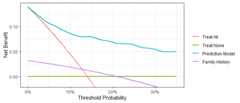
Time-to-event or survival endpoints
dca(Surv(ttcancer, cancer)~ cancerpredmarker,data = df_surv,time =1,thresholds =seq(0,0.50,by =0.01),label =list(cancerpredmarker ="Prediction Model"))%>%plot(smooth =TRUE)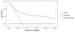
Create a customized DCA figure by first printing the ggplot code.Copy and modify the ggplot code as needed.
gg_dca<-dca(cancer~ cancerpredmarker,data = df_binary,thresholds =seq(0,0.35,by =0.01),label =list(cancerpredmarker ="Prediction Model"))%>%plot(smooth =TRUE,show_ggplot_code =TRUE)#> # ggplot2 code to create DCA figure -------------------------------#> as_tibble(x) %>%#> dplyr::filter(!is.na(net_benefit)) %>%#> ggplot(aes(x = threshold, y = net_benefit, color = label)) +#> stat_smooth(method = "loess", se = FALSE, formula = "y ~ x",#> span = 0.2) +#> coord_cartesian(ylim = c(-0.014, 0.14)) +#> scale_x_continuous(labels = scales::percent_format(accuracy = 1)) +#> labs(x = "Threshold Probability", y = "Net Benefit", color = "") +#> theme_bw()Pfeiffer, Ruth M, and Mitchell H Gail. (2020) “Estimating theDecision Curve and Its Precision from Three Study Designs.”Biometrical Journal 62 (3): 764–76.
Vickers, Andrew J, Angel M Cronin, Elena B Elkin, and Mithat Gonen.(2008)“Extensions to Decision Curve Analysis, a Novel Method forEvaluating Diagnostic Tests, Prediction Models and Molecular Markers.”BMC Medical Informatics and Decision Making 8 (1): 1–17.
Vickers, Andrew J, and Elena B Elkin. (2006) “Decision CurveAnalysis: A Novel Method for Evaluating Prediction Models.”MedicalDecision Making 26 (6): 565–74.