Movatterモバイル変換

Targeted Learning in R(targeted)

Various methods for targeted learning and semiparametric inferenceincluding augmented inverse probability weighted (AIPW) estimators formissing data and causal inference (Bang and Robins (2005)doi:10.1111/j.1541-0420.2005.00377.x), variableimportance and conditional average treatment effects (CATE) (van derLaan (2006)doi:10.2202/1557-4679.1008), estimators for riskdifferences and relative risks (Richardson et al. (2017)doi:10.1080/01621459.2016.1192546), assumption leaninference for generalized linear model parameters (Vansteelandt etal. (2022)doi:10.1111/rssb.12504).

Installation

You can install the released version of targeted fromCRAN with:

install.packages("targeted")

And the development version fromGitHub with:

remotes::install_github("kkholst/targeted",ref="dev")

Computations such as cross-validation are parallelized via the{future} package. To enable parallel computations andprogress-bars the following code can be executed

future::plan("multisession")progressr::handlers(global=TRUE)

Examples

To illustrate some of the functionality of thetargetedpackage we simulate some data from the following model\[Y = \exp\{-(W_1 - 1)^2 - (W_2 - 1)^2)\} -2\exp\{-(W_1+1)^2 - (W_2+1)^2\}A + \epsilon\] with independentmeasurement error\(\epsilon\sim\mathcal{N}(0,1)\), treatmentvariable\(A \simBernoulli(\text{expit}\{-1+W_1\})\) and independent covariates\(W_1, W_2\sim\mathcal{N}(0,1/2)\).

library("targeted")simdata<-function(n, ...) {   w1<-rnorm(n)# covariates   w2<-rnorm(n)# ...   a<-rbinom(n,1,plogis(-1+ w1))# treatment indicator   y<-exp(- (w1-1)**2- (w2-1)**2)-# continuous response2*exp(- (w1+1)**2- (w2+1)**2)* a+# additional effect in treatedrnorm(n,sd=0.5**.5)data.frame(y, a, w1, w2)}set.seed(1)d<-simdata(5e3)head(d)#>             y a         w1         w2#> 1 -0.59239667 0 -0.6264538 -1.5163733#> 2  0.01794935 0  0.1836433  0.6291412#> 3  0.24968229 0 -0.8356286 -1.6781940#> 4  1.34434300 1  1.5952808  1.1797811#> 5  1.16367655 0  0.3295078  1.1176545#> 6 -0.94757031 0 -0.8204684 -1.2377359

wnew<-seq(-3,3,length.out=200)dnew<-expand.grid(w1 = wnew,w2 = wnew,a =1)y<-with(dnew,exp(- (w1-1)**2- (w2-1)**2)-2*exp(- (w1+1)**2- (w2+1)**2)*a          )image(wnew, wnew,matrix(y,ncol=length(wnew)),col=viridisLite::viridis(64),main=expression(paste("E(Y|",W[1],",",W[2],")")),xlab=expression(W[1]),ylab=expression(W[2]))

Nuisance (prediction) models

Methods for targeted and semiparametric inference rely on fittingnuisance models to observed data when estimating the target parameter ofinterest. The{targeted} package implements theR6 reference classlearnerto harmonize common statistical and machine learning models for theusage as nuisance models across the various implemented estimators, suchas thetargeted:cate function. Commonly used models areconstructed aslearner class objects through thelearner_* functions.

As an example, we can specify a linear regression model with aninteraction term between treatment and the two covariates\(W_1\) and\(W_2\)

lr<-learner_glm(y~ (w1+ w2)*a,family = gaussian)lr#> ────────── learner object ──────────#> glm#>#> Estimate arguments: family=<function>#> Predict arguments:#> Formula: y ~ (w1 + w2) * a <environment: 0xaee788b30>

To fit the model to the data we use theestimatemethod

lr$estimate(d)lr$fit#>#> Call:  stats::glm(formula = formula, family = family, data = data)#>#> Coefficients:#> (Intercept)           w1           w2            a         w1:a         w2:a#>     0.18808      0.13044      0.08253     -0.33517      0.15330      0.24068#>#> Degrees of Freedom: 4999 Total (i.e. Null);  4994 Residual#> Null Deviance:       3098#> Residual Deviance: 2741  AIC: 11200

Predictions,\(E(Y\mid W_1, W_2)\),can be performed with thepredict method

head(d)|> lr$predict()#>           1           2           3           4           5           6#> -0.01878799  0.26395942 -0.05942914  0.68687155  0.32330487 -0.02109944

pr<-matrix(lr$predict(dnew),ncol=length(wnew))image(wnew, wnew, pr,col=viridisLite::viridis(64),main=expression(paste("E(Y|",W[1],",",W[2],")")),xlab=expression(W[1]),ylab=expression(W[2]))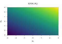

Similarly, a Random Forest can be specified with

lr_rf<-learner_grf(y~ w1+ w2+ a,num.trees =500)

Lists of models can also be constructed for differenthyper-parameters with thelearner_expand_grid function.

Cross-validation

To assess the model generalization error we can perform\(k\)-fold cross-validation with thecv method

mod<-list(glm = lr,rf = lr_rf)cv(mod,data = d,rep =2,nfolds =5)|>summary()#> , , mse#>#>          mean         sd       min       max#> glm 0.5498117 0.02987117 0.5085057 0.5969734#> rf  0.5070569 0.03177828 0.4597520 0.5534290#>#> , , mae#>#>          mean         sd       min       max#> glm 0.5907746 0.01516298 0.5686472 0.6148165#> rf  0.5684956 0.01659710 0.5453521 0.5953637

Ensembles (Super-Learner)

An ensemble learner (super-learner) can easily be constructed fromlists oflearner objects

sl<-learner_sl(mod,nfolds =10)sl$estimate(d)sl#> ────────── learner object ──────────#> superlearner#>  glm#>  rf#>#> Estimate arguments: learners=<list>, nfolds=10, meta.learner=<function>, model.score=<function>#> Predict arguments:#> Formula: y ~ (w1 + w2) * a <environment: 0x15cf956c8>#> ─────────────────────────────────────#>         score     weight#> glm 0.5499084 0.03290729#> rf  0.5070931 0.96709271

pr<-matrix(sl$predict(dnew),ncol=length(wnew))image(wnew, wnew, pr,col=viridisLite::viridis(64),main=expression(paste("E(Y|",W[1],",",W[2],")")),xlab=expression(W[1]),ylab=expression(W[2]))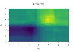

Average Treatment Effects

In the following we are interested in estimating the target parameter\(\psi_a(P) = E_P[Y(a)]\), where\(Y(a)\) is thepotential outcome wewould have observed if treatment\(a\)had been administered, possibly contrary to the actual treatment thatwas observed, i.e.,\(Y = Y(A)\). Toassess the treatment effect we can then the consider theaveragetreatment effect (ATE)\[E_P[Y(1)]-E_P[Y(0)],\] or some othercontrast of interest\(g(\psi_1(P),\psi_0(P))\). Under the following assumptions

1. Stable Unit Treatment Values Assumption (the treatment of a specificsubject is not affecting the potential outcome of other subjects)
2. Positivity,\(P(A\midW)>\epsilon\) for some\(\epsilon>0\) and baseline covariates\(W\)
3. No unmeasured confounders,\(Y(a)\perp\!\!\! \perp A|W\)

then the target parameter can be identified from the observed datadistribution as\[E(E[Y|W,A=a]) =E(E[Y(a)|W]) = E[Y(a)]\] or\[E[YI(A=a)/P(A=a|W)] = E[Y(a)].\]

This suggests estimators based on outcome regression (\(g\)-computation) or inverse probabilityweighting. More generally, under the above assumption we can constructoraone-step estimator from theEfficient InfluenceFunction combining these two\[E\left[\frac{I(A=a)}{\Pi_a(W)}(Y-Q(W,A)) + Q(W,a)\right].\]
In practice, this requires plugin estimates of both the outcome model,\(Q(W,A) := E(Y\mid A, W)\), and of thetreatment propensity model\(\Pi_a(W) :=P(A=a\mid W)\). The corresponding estimator is consistent even ifjust one of the two nuisance models is correctly specified.

First we specify the propensity model

prmod<-learner_glm(a~ w1+ w2,family=binomial)

We will reuse one of the outcome models from the previous section,and use thecate function to estimate the treatmenteffect

a<-cate(response.model = lr_rf,propensity.model = prmod,data = d,nfolds =5)a#>             Estimate Std.Err       2.5%   97.5%   P-value#> E[y(1)]      -0.1700 0.02628 -0.2214840 -0.1185 9.939e-11#> E[y(0)]       0.1483 0.07595 -0.0005763  0.2971 5.089e-02#> ───────────#> (Intercept)  -0.3183 0.07996 -0.4749849 -0.1615 6.892e-05

In the output we get estimates of both the mean potential outcomesand the difference of those, the average treatment effect, given as theterm(Intercept).

summary(a)#> cate(response.model = lr_rf, propensity.model = prmod, data = d,#>     nfolds = 5)#>#>             Estimate Std.Err       2.5%   97.5%   P-value#> E[y(1)]      -0.1700 0.02628 -0.2214840 -0.1185 9.939e-11#> E[y(0)]       0.1483 0.07595 -0.0005763  0.2971 5.089e-02#> ───────────#> (Intercept)  -0.3183 0.07996 -0.4749849 -0.1615 6.892e-05#>#> Average Treatment Effect:#>                       Estimate Std.Err    2.5%   97.5%   P-value#> [E[y(1)]] - [E[y(0)]]  -0.3183 0.08008 -0.4752 -0.1613 7.055e-05#>#>  Null Hypothesis:#>   [E[y(1)]] - [E[y(0)]] = 0

Here we use thenfolds=5 argument to use 5-foldcross-fitting to guarantee that the estimates converges weaklyto a Gaussian distribution even though that the estimated influencefunction based on plugin estimates from the Random Forest does notnecessarily lie in a\(P\)-Donskerclass.

Project organization

We use thedev branch for development and themain branch for stable releases. All releases followsemantic versioning, aretagged and notablechanges are reported inNEWS.md.

I Have a Question / IWant to Report a Bug

If you want to ask questions, require help or clarification, orreport a bug, we recommend to either contact a maintainer directly orthe following:

• Open anIssue.
• Provide as much context as you can about what you’re runninginto.
• Provide project and platform versions, depending on what seemsrelevant.

We will then take care of the issue as soon as possible.

Contributing totargeted

All types of contributions are encouraged and valued. See theCONTRIBUTING.mdfor details about how to contribute code to this project.