Movatterモバイル変換

cpam(changepointadditivemodels)

An R package foromics time series analysis.

Read the methods paperhere

Application ofcpam to RNA-seq time series ofArabidopsis plants treated with excess-light.

Key features

• Changepoint detection: Identify sharp transitionsin expression.
• smooth trends: Model expression as a smoothfunction of time.
• Shape-constrained trends: Cluster targets intobiologically meaningful temporal shape classes.
• Quantification uncertainty: Account for uncertaintyin expression estimates.
• Transcript-level analysis
  • Perform gene- or transcript-level inferences.
  • Aggregate\(p\)-values at the genelevel for improved power.
• Case-only or case-control time series: Analyse timeseries data with or without controls.
• User-friendly: Sensible defaults and an interactiveshiny interface.

Our new packagecpam provides a comprehensiveframework for analysing time series omics data. The method uses modernstatistical approaches while remaining user-friendly, through sensibledefaults and an interactive interface. Researchers can directly addresskey questions in time series analysis—when changes occur, what patternsthey follow, and how responses are related. While we have focused ontranscriptomics, the framework is applicable to other high-dimensionaltime series measurements.

If you encounter issues or have suggestions for improvements, pleaseopen anissue. Wewelcome questions and discussion about usingcpam foryour research throughDiscussions.Our goal is to work with users to makecpam a robustand valuable tool for time series omics analysis. We can also becontacted via the email addresses listed in our paperhere.

Installation

The package is available on CRAN and can be installed using thefollowing command:

install.packages("cpam")

Usage

Step 1: Load the package

library(cpam)

Step 2:Create a tibble for the experimental design.

In thisArabidopsis thaliana time series example, we usedthe softwarekallisto togenerate counts from RNA-seq data. To load the counts, we provide thefile path for each kallisto output file (alternatively you can providethe counts directly as count matrix, or use other quantificationsoftware)

# load example dataload(system.file("extdata","exp_design_path.rda",package ="cpam"))head(exp_design_path)#>   sample time                                path condition#> 1 JHSS01    0 output/kallisto/JHSS01/abundance.h5 treatment#> 2 JHSS02    0 output/kallisto/JHSS02/abundance.h5 treatment#> 3 JHSS03    0 output/kallisto/JHSS03/abundance.h5 treatment#> 4 JHSS04    0 output/kallisto/JHSS04/abundance.h5 treatment#> 5 JHSS05    0 output/kallisto/JHSS05/abundance.h5 treatment#> 6 JHSS06    5 output/kallisto/JHSS06/abundance.h5 treatment

Step3: Obtain a table with the transcript-to-gene mapping

N.B. This is not needed if your counts are aggregated at the genelevel, but transcript-level analysis with aggregation of\(p\)-values to the gene level isrecommended. E.g., forArabidopsis thaliana:

# load example dataload(system.file("extdata","t2g_arabidopsis.rda",package ="cpam"))head(t2g_arabidopsis)#>     target_id   gene_id#> 1 AT1G01010.1 AT1G01010#> 2 AT1G01020.2 AT1G01020#> 3 AT1G01020.6 AT1G01020#> 4 AT1G01020.1 AT1G01020#> 5 AT1G01020.4 AT1G01020#> 6 AT1G01020.5 AT1G01020

Step 4: Runcpam

  cpo<-prepare_cpam(exp_design = exp_design_path,count_matrix =NULL,t2g = t2g_arabidopsis,model ="case-only",import_type ="kallisto",num_cores =5)  cpo<-compute_p_values(cpo)  cpo<-estimate_changepoint(cpo)  cpo<-select_shape(cpo)

Step 5: Visualise the results

Load the shiny app for an interactive visualisation of theresults:

visualise(cpo)# not shown in vignette

Or plot one gene at a time:

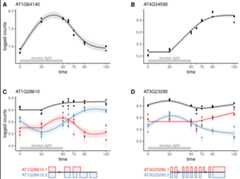
plot_cpam(cpo,gene_id ="AT3G23280")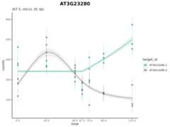

Isoform 1 (AT3G23280.1) has a changepoint at 67.5 min and has amonotonic increasing concave (micv) shape. Isoform 2 (AT3G23280.2) hasno changepoint and has an unconstrained thin-plate (tp) shape.

We can generate a results table which has\(p\)-values, shapes, log-fold changes andcounts with many optimal filters (see tutorials):

results(cpo)#> # A tibble: 15,279 × 25#>    target_id   gene_id     p    cp shape lfc.0 lfc.5 lfc.10 lfc.20 lfc.30 lfc.45#>    <chr>       <chr>   <dbl> <dbl> <chr> <dbl> <dbl>  <dbl>  <dbl>  <dbl>  <dbl>#>  1 AT1G01910.1 AT1G01…     0     0 micv      0 1.01   1.70   2.38   2.60   2.73#>  2 AT1G01910.2 AT1G01…     0    10 cv        0 0      0      0.553  0.775  0.790#>  3 AT1G01910.5 AT1G01…     0    10 cx        0 0      0     -3.20  -4.57  -4.82#>  4 AT1G02610.1 AT1G02…     0    45 mdcx      0 0      0      0      0      0#>  5 AT1G02610.2 AT1G02…     0    10 cx        0 0      0     -0.645 -1.16  -1.71#>  6 AT1G02610.3 AT1G02…     0    10 mdcx      0 0      0     -1.48  -2.11  -2.25#>  7 AT1G04080.1 AT1G04…     0    10 cv        0 0      0      2.75   3.85   3.97#>  8 AT1G04080.2 AT1G04…     0    45 micv      0 0      0      0      0      0#>  9 AT1G04080.3 AT1G04…     0     0 micv      0 0.268  0.445  0.603  0.638  0.656#> 10 AT1G04080.5 AT1G04…     0    10 cx        0 0      0     -2.17  -3.04  -3.10#> # ℹ 15,269 more rows#> # ℹ 14 more variables: lfc.60 <dbl>, lfc.90 <dbl>, lfc.180 <dbl>,#> #   lfc.240 <dbl>, counts.0 <dbl>, counts.5 <dbl>, counts.10 <dbl>,#> #   counts.20 <dbl>, counts.30 <dbl>, counts.45 <dbl>, counts.60 <dbl>,#> #   counts.90 <dbl>, counts.180 <dbl>, counts.240 <dbl>

Tutorials

For a quick-to-run introductory example, we have provided a smallsimulated data set as part of the package.

• IntroductoryExample

The following two tutorials use real-world data to demonstrate thecapabilities of thecpam package. In addition, theyprovide code to reproduce the results for the case studies presented inthemanuscriptaccompanying thecpam package.

• ArabidopsisCase Study
• HumanEmbryo Case Study

Acknowledgements

This work was supported by the Australian Research Council, Centre ofExcellence for Plant Success in Nature and Agriculture(CE200100015).