


The goal of expstudy is to provide a set of tools to quickly conductanalysis of an experience study. Commonly used techniques (such asactual-to-expected analysis) are generalized and streamlined so thatrepetitive coding is avoided.
Most analyses for an experience study is structured aroundmeasures for a particular decrement of interest, e.g., thenumber of policy surrenders for a surrender experience study. For anygiven decrement of interest, the following measures are commonlyutilized:
expstudy provides functions to recognize or identify study measuresso that the routine analyses can be streamlined.
expstudy is published to CRAN so you can download directly from anyCRAN mirror:
install.packages('expstudy')To get a bug fix or to use a feature from the development version,you can install the development version of expstudy from GitHub.
# Uncomment below if you do not have pak installed yet.# install.packages('pak')pak::pak('cb12991/expstudy')library(expstudy)This package provides a sample mortality experience study to aid withexamples:
dplyr::glimpse(mortexp)#> Rows: 176,096#> Columns: 23#> $ AS_OF_DATE <date> 1998-04-30, 1998-05-31, 1998-06-30, 1998-07-31,…#> $ POLICY_HOLDER <fct> PH_0001, PH_0001, PH_0001, PH_0001, PH_0001, PH_…#> $ GENDER <fct> FEMALE, FEMALE, FEMALE, FEMALE, FEMALE, FEMALE, …#> $ SMOKING_STATUS <fct> NON-SMOKER, NON-SMOKER, NON-SMOKER, NON-SMOKER, …#> $ UNDERWRITING_CLASS <fct> STANDARD, STANDARD, STANDARD, STANDARD, STANDARD…#> $ FACE_AMOUNT <dbl> 5000, 5000, 5000, 5000, 5000, 5000, 5000, 5000, …#> $ INSURED_DOB <date> 1977-01-20, 1977-01-20, 1977-01-20, 1977-01-20,…#> $ ISSUE_DATE <date> 1998-04-02, 1998-04-02, 1998-04-02, 1998-04-02,…#> $ TERMINATION_DATE <date> 2013-08-08, 2013-08-08, 2013-08-08, 2013-08-08,…#> $ ISSUE_AGE <dbl> 20, 20, 20, 20, 20, 20, 20, 20, 20, 20, 20, 20, …#> $ ATTAINED_AGE <dbl> 22, 22, 22, 22, 22, 22, 22, 22, 22, 23, 23, 23, …#> $ EXPECTED_MORTALITY_RT <dbl> 0.01020408, 0.01020408, 0.01020408, 0.01020408, …#> $ POLICY_DURATION_YR <dbl> 1, 1, 1, 1, 1, 1, 1, 1, 1, 1, 1, 1, 2, 2, 2, 2, …#> $ POLICY_DURATION_MNTH <int> 1, 2, 3, 4, 5, 6, 7, 8, 9, 10, 11, 12, 13, 14, 1…#> $ POLICY_STATUS <fct> SURRENDERED, SURRENDERED, SURRENDERED, SURRENDER…#> $ MORT_EXPOSURE_CNT <dbl> 0.07671233, 0.08219178, 0.07945205, 0.08219178, …#> $ MORT_EXPOSURE_AMT <dbl> 383.5616, 410.9589, 397.2603, 410.9589, 410.9589…#> $ MORT_ACTUAL_CNT <dbl> 0, 0, 0, 0, 0, 0, 0, 0, 0, 0, 0, 0, 0, 0, 0, 0, …#> $ MORT_ACTUAL_AMT <dbl> 0, 0, 0, 0, 0, 0, 0, 0, 0, 0, 0, 0, 0, 0, 0, 0, …#> $ MORT_EXPECTED_CNT <dbl> 0.0007827789, 0.0008386916, 0.0008107353, 0.0008…#> $ MORT_EXPECTED_AMT <dbl> 3.913894, 4.193458, 4.053676, 4.193458, 4.193458…#> $ MORT_VARIANCE_CNT <dbl> 0.0007821661, 0.0008379882, 0.0008100780, 0.0008…#> $ MORT_VARIANCE_AMT <dbl> 19554.15, 20949.71, 20251.95, 20949.71, 20949.71…Assumptions within an experience study are often evaluated viaactual-to-expected (AE) ratios. The aggregate assumption performance canbe reviewed by totaling up the actuals and dividing by the totalexpecteds to produce the AE ratio. An AE ratio close to 100% signifiesthe expectation using the underlying assumption reflects actualpolicyholder behavior observed in experience.
Calculating the aggregate AE ratio without expstudy (with the help ofthe tidyverse/dplyr package) is shown below:
library(dplyr)mortexp%>%summarise(across(.cols =c( MORT_EXPOSURE_CNT, MORT_ACTUAL_CNT, MORT_EXPECTED_CNT, MORT_VARIANCE_CNT, MORT_EXPOSURE_AMT, MORT_ACTUAL_AMT, MORT_EXPECTED_AMT, MORT_VARIANCE_AMT ),.fns = \(x)sum(x,na.rm =TRUE) ) )%>%mutate(CNT_AE_RATIO = MORT_ACTUAL_CNT/ MORT_EXPECTED_CNT,AMT_AE_RATIO = MORT_ACTUAL_AMT/ MORT_EXPECTED_AMT )%>% glimpse#> Rows: 1#> Columns: 10#> $ MORT_EXPOSURE_CNT <dbl> 14295.43#> $ MORT_ACTUAL_CNT <dbl> 315#> $ MORT_EXPECTED_CNT <dbl> 256.4227#> $ MORT_VARIANCE_CNT <dbl> 255.9583#> $ MORT_EXPOSURE_AMT <dbl> 210257356#> $ MORT_ACTUAL_AMT <dbl> 4650000#> $ MORT_EXPECTED_AMT <dbl> 3843358#> $ MORT_VARIANCE_AMT <dbl> 148007176380#> $ CNT_AE_RATIO <dbl> 1.22844#> $ AMT_AE_RATIO <dbl> 1.20988Using expstudy, the code to produce the same output is asfollows:
mortexp%>% summarise_measures%>% mutate_metrics%>% glimpse#> Rows: 1#> Columns: 18#> $ MORT_ACTUAL_CNT <dbl> 315#> $ MORT_EXPOSURE_CNT <dbl> 14295.43#> $ MORT_EXPECTED_CNT <dbl> 256.4227#> $ MORT_VARIANCE_CNT <dbl> 255.9583#> $ MORT_ACTUAL_AMT <dbl> 4650000#> $ MORT_EXPOSURE_AMT <dbl> 210257356#> $ MORT_EXPECTED_AMT <dbl> 3843358#> $ MORT_VARIANCE_AMT <dbl> 148007176380#> $ AVG_OBSRV_CNT <dbl> 0.02203501#> $ AVG_EXPEC_CNT <dbl> 0.01793739#> $ CI_FCTR_CNT <dbl> 0.002193488#> $ AE_RATIO_CNT <dbl> 1.22844#> $ CREDIBILITY_CNT <dbl> 0.4088781#> $ AVG_OBSRV_AMT <dbl> 0.02211575#> $ AVG_EXPEC_AMT <dbl> 0.0182793#> $ CI_FCTR_AMT <dbl> 0.003586231#> $ AE_RATIO_AMT <dbl> 1.20988#> $ CREDIBILITY_AMT <dbl> 0.2548539The runtimes of each do not significantly differ, so there is noperformance degradation with the code improvement:
library(microbenchmark)library(ggplot2)autoplot(microbenchmark(dplyr_only = mortexp%>%summarise(across(.cols =c( MORT_EXPOSURE_CNT, MORT_ACTUAL_CNT, MORT_EXPECTED_CNT, MORT_VARIANCE_CNT, MORT_EXPOSURE_AMT, MORT_ACTUAL_AMT, MORT_EXPECTED_AMT, MORT_VARIANCE_AMT ),.fns = \(x)sum(x,na.rm =TRUE) ) )%>%mutate(CNT_AE_RATIO = MORT_ACTUAL_CNT/ MORT_EXPECTED_CNT,AMT_AE_RATIO = MORT_ACTUAL_AMT/ MORT_EXPECTED_AMT ),expstudy = mortexp%>% summarise_measures%>% mutate_metrics))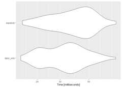
Note that expstudy is calculating more than the AE ratio metric.Without those additional metrics, performance with expstudy actuallysurpasses performance without:
autoplot(microbenchmark(dplyr_only = mortexp%>%summarise(across(.cols =c( MORT_EXPOSURE_CNT, MORT_ACTUAL_CNT, MORT_EXPECTED_CNT, MORT_VARIANCE_CNT, MORT_EXPOSURE_AMT, MORT_ACTUAL_AMT, MORT_EXPECTED_AMT, MORT_VARIANCE_AMT ),.fns = \(x)sum(x,na.rm =TRUE) ) )%>%mutate(CNT_AE_RATIO = MORT_ACTUAL_CNT/ MORT_EXPECTED_CNT,AMT_AE_RATIO = MORT_ACTUAL_AMT/ MORT_EXPECTED_AMT ),expstudy = mortexp%>% summarise_measures%>%mutate_metrics(metrics =list(AE_RATIO = ae_ratio) )))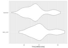
Whenever there is not enough credibility for a company to write theirown assumption, adjustment factors are often used to incorporateemerging experience. expstudy provides a function to determine factoradjustments for each provided set of measures using a variety ofmethods.
mortexp%>%group_by( GENDER, SMOKING_STATUS )%>%compute_fct_adjs(expected_rate = EXPECTED_MORTALITY_RT,amount_scalar = FACE_AMOUNT,method ='sequential' )#> $CNT#> SMOKING_STATUS GENDER GENDER_FCT_ADJ SMOKING_STATUS_FCT_ADJ COMPOSITE_FCT_ADJ#> 1 NON-SMOKER FEMALE 1.271511 1.0194734 1.296272#> 2 NON-SMOKER MALE 1.193514 1.0194734 1.216755#> 3 SMOKER FEMALE 1.271511 0.9515988 1.209968#> 4 SMOKER MALE 1.193514 0.9515988 1.135746#>#> $AMT#> SMOKING_STATUS GENDER GENDER_FCT_ADJ SMOKING_STATUS_FCT_ADJ COMPOSITE_FCT_ADJ#> 1 NON-SMOKER FEMALE 1.307949 0.998288 1.305710#> 2 NON-SMOKER MALE 1.129454 0.998288 1.127520#> 3 SMOKER FEMALE 1.307949 1.004059 1.313259#> 4 SMOKER MALE 1.129454 1.004059 1.134039Refer to each function’s documentation page for additionaldetail.
Please note that the expstudy project is released with aContributorCode of Conduct. By contributing to this project, you agree to abideby its terms.