
This package provides a pipeline for short tandem repeat instabilityanalysis from fragment analysis data. The inputs are fsa files or peaktables (e.g. Genemapper 5 software peak table output), and a usersupplied metadata data-frame. The functions identify ladders, callspeaks, and calculate repeat instability metrics (i.e. expansion index oraverage repeat gain).
This code is not for clinical use. There are features for accuraterepeat sizing if you use validated control samples, but integer repeatunits are not returned.
To report bugs or feature requests, please visit the Github issuetrackerhere. Forassistance or any other inquires, contactZach McLean.
If you use this package, please citethis paperfor now.
How to use the package
For an easy way to get started with your own data or to run anexample, usetrace::generate_trace_template() to generate adocument with the pipeline pre-populated.
In this package, each sample is represented by an R6 ‘fragments’object, which are organized in lists. Functions in the package iterateover these lists, so you usually don’t need to interact with the objectsdirectly. If you do, the attributes of the objects can be accessed with$, and note that most functions modify the objects in place, sore-assignment isn’t necessary. The only exception to thatfind_fragments(), which transitions to a new object sincethe class structure changes.
There are several important factors to a successful repeatinstability experiment and things to consider when using thispackage:
(required) Each sample has a unique id, usually the filename
(optional) Baseline control for your experiment. For example,specifying a sample where the modal allele is the inherited repeatlength (eg a mouse tail sample) or a sample at the start of atime-course experiment. This is indicated with a
TRUEinthemetrics_baseline_controlcolumn of the metadata.Samples are then grouped together with themetrics_group_idcolumn of the metadata. Multiple samples can bemetrics_baseline_control, which can be helpful for theaverage repeat gain metric to have a more accurate representation of theaverage repeat at the start of the experiment.(optional) Batch or repeat length correction for systematic batcheffects that occur with repeat-containing amplicons in capillaryelectrophoresis.
Repeat containing amplicons do not run linearly with internalladder sizes in capillary electrophoresis resulting is anunderestimation of repeat length if you just convert from base-pairsize. These differences are not always consistent across runs which canresult in batch effects in the repeat size. So, if the repeat length isto be directly compared for samples from different runs, this batcheffect needs to be corrected. This is only relevant when the absolutesize of a amplicons are compared for grouping metrics as described above(otherwise instability metrics are all relative and it doesn’t matterthat there’s systematic batch effects across runs), when plotting tracesfrom different runs, or if an accurate repeat length isdesired.
There are two main correction approaches that are somewhatrelated: either ‘batch’ or ‘repeat’ in
call_repeats().Batch correction is relatively simple and just requires you to linksamples across batches by indicating them from metadata. But even thoughthe repeat size that is return will be precise, it will not be accurateand underestimates the real repeat length. By contrast, repeatcorrection can be used to accurately call repeat lengths (which alsocorrects the batch effects). However, the repeat correction will only beas good as your sample(s) used to call the repeat length, so this can achallenging and advanced feature. You need to use a sample that reliablyreturns the same peak as the modal peak, or you need to be willing tounderstand the shape of the distribution and manually validate therepeat length of each control sample for each run.
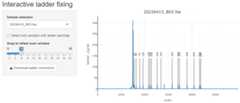
If starting from fsa files, the GeneScan™ 1200 LIZ™ dye SizeStandard ladder assignment may not work very well. The ladderidentification algorithm is optimized for GeneScan™ 500 LIZ™ orGeneScan™ 600 LIZ™ or other ladders with relatively few peaks. The 1200LIZ™ ladder has a challenging pattern of ladder peaks to automaticallyassign. However, these ladders can be fixed by playing with the variousparameters or manually with the built-in fix_ladders_interactive()app.
Installation
Install the package from CRAN:
install.packages("trace")Development version
You can install the development version fromGitHub with:
if (!require("pak",quietly =TRUE))install.packages("pak")pak::pak("zachariahmclean/trace")Import data
Load the package:
library(trace)First, we read in the raw data. In this case we will used exampledata within this package, but usually this would be fsa files that areread in usingread_fsa(). The example data is also clonedsince the next step modifies the object in place.
fsa_list<-lapply(cell_line_fsa_list,function(x) x$clone())Find ladders
The known ladder sizes are assigned to peaks in the ladder channeland bp are predicted for each scan.
find_ladders( fsa_list,show_progress_bar =FALSE)visually inspect each ladder to make sure that the ladders werecorrectly assigned
plot_ladders(fsa_list[1])
If the ladders are are not assigned correctly, you can adjustparameters or manually using the built-in fix_ladders_interactive()app.
Find fragments
The fragment peaks are identified in the raw continuous trace data.These objects are assigned because find_fragments transitions to a newobject since the class structure changes. This reflects the data movingfrom a continuous trace to a peak table.
fragments_list<-find_fragments( fsa_list,min_bp_size =300)Visually inspect the traces and called peaks to make sure they werecorrectly assigned.
plot_traces(fragments_list[1],xlim =c(400,550),ylim =c(0,1200))
Alternatively, this is where you would use data exported fromGenemapper if you would rather use the Genemapper bp sizing and peakidentification algorithms. However, this is not recommended as some ofthe functionality of this package would not be accessible (mainly incall_repeats(), withbatch_correction andrepeat calling algorithms)
fragments_list_genemapper<-peak_table_to_fragments(example_data,data_format ="genemapper5",dye_channel ="B",min_size_bp =300)Add metadata
Metadata can be incorporated to allow additional functionality incall_repeats() (batch or repeat correction) andassign_index_peaks() (assigning index peak from anothersample). Prepare a file (eg spreadsheet saved as .csv) with thefollowing columns. If you use the specified column names, it will beautomatically parsed byadd_metadata(), otherwise you willneed to match up which column name belongs to which metadata category(as done below inadd_metadata()):
| Metadata table column | Functionality metadata is associated with | Description |
|---|---|---|
| unique_id | Required for adding metadata usingadd_metadata() | The unique identifier for the fsa file. Usually the sample filename. This must be unique, including across runs. |
| metrics_group_id | assign_index_peaks(), allows settinggrouped | This groups the samples for instability metric calculations. Providea group id value for each sample. For example, in a mouse experiment andusing the expansion index, you need to group the samples since they havethe same metrics baseline control (eg inherited repeat length), soprovide the mouse id. |
| metrics_baseline_control | assign_index_peaks(), allows settinggrouped | This is related to metrics_group_id. Indicate with ‘TRUE’ to specifywhich sample is the baseline control (eg mouse tail for inherited repeatlength, or day-zero sample in cell line experiments) |
| batch_run_id | call_repeats(), allows settingcorrection= “batch” or “repeat” | This groups the samples by batch. Provide a value for each fragmentanalysis run (eg date). |
| batch_sample_id | call_repeats(), allows settingcorrection= “batch” or “repeat” | This groups the samples across batches. Give a unique sample id toeach different sample. |
| batch_sample_modal_repeat | call_repeats(), allows settingcorrection= “repeat” | The validated modal repeat length for the particularbatch_sample_id sample used to accurately call repeatlength. |
add_metadata(fragments_list = fragments_list,metadata_data.frame = metadata,unique_id ="unique_id",metrics_group_id ="metrics_group_id",metrics_baseline_control ="metrics_baseline_control",batch_run_id ="batch_run_id",batch_sample_id ="batch_sample_id",batch_sample_modal_repeat ="batch_sample_modal_repeat")Identify modal peaks andcall repeats
Next we identify the modal peaks withfind_alleles() andconvert the base pair fragments to repeats withcall_repeats().
find_alleles(fragments_list)call_repeats(fragments_list)We can view the distribution of repeat sizes and the identified modalpeak with a plotting function.
plot_traces(fragments_list[1],xlim =c(110,150))
Assign index peaks
A key part of several instability metrics is the index peak. This isthe repeat length used as the reference for relative instability metricscalculations, like expansion index or average repeat gain. In themetadata, samples are grouped by ametrics_group_id and asubset of the samples are set asmetrics_baseline_control,meaning they are the samples taken at day 0 in this experiment. Thisallows us to setgrouped = TRUE and set the index peak forthe expansion index and other metrics. For mice, if just a few sampleshave the inherited repeat signal shorter than the expanded population,you could not worry about this and instead use theindex_override_dataframe inassign_index_peaks().
assign_index_peaks( fragments_list,grouped =TRUE)We can validate that the index peaks were assigned correctly with adotted vertical line added to the trace. This is perhaps more useful inthe context of mice where you can visually see when the inherited repeatlength should be in the bimodal distribution.
plot_traces(fragments_list[1],xlim =c(110,150))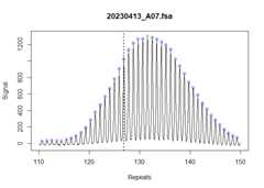
Calculate instabilitymetrics
All of the information we need to calculate the repeat instabilitymetrics has now been identified. We can finally usecalculate_instability_metrics to generate a dataframe ofper-sample metrics.
metrics_grouped_df<-calculate_instability_metrics(fragments_list = fragments_list,peak_threshold =0.05,window_around_index_peak =c(-40,40))These metrics can then be used to quantify repeat instability. Forexample, this reproduces a subset of Figure 7e ofourmanuscript.
library(ggplot2)library(dplyr)#>#> Attaching package: 'dplyr'#> The following objects are masked from 'package:stats':#>#> filter, lag#> The following objects are masked from 'package:base':#>#> intersect, setdiff, setequal, unionmetrics_grouped_df|>left_join(metadata,by =join_by(unique_id))|>filter( day>0, modal_peak_signal>500 )|>ggplot(aes(as.factor(treatment), average_repeat_change))+geom_boxplot()+geom_jitter()+labs(y ="Average repeat gain",x ="Branaplam (nM)")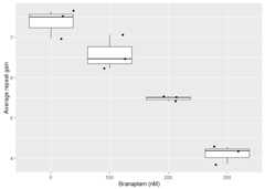
[8]ページ先頭