


holodeck allows quick and simple creation of simulatedmultivariate data with variables that co-vary or discriminate betweenlevels of a categorical variable. The resulting simulated multivariatedataframes are useful for testing the performance of multivariatestatistical techniques under different scenarios, power analysis, orjust doing a sanity check when trying out a new multivariate method.
From CRAN:
install.packages("holodeck)Development version from r-universe:
install.packages('holodeck',repos =c('https://aariq.r-universe.dev','https://cloud.r-project.org'))holodeck is built to work withdplyrfunctions, includinggroup_by() and the pipe(%>%).purrr is helpful for iteratingsimulated data. For these examples I’ll useropls for PCAand PLS-DA.
library(holodeck)library(dplyr)library(tibble)library(purrr)library(ropls)Let’s say we want to learn more about how principal componentanalysis (PCA) works. Specifically, what matters more in terms ofcreating a principal component—variance or covariance of variables? Tothis end, you might create a dataframe with a few variables with highcovariance and low variance and another set of variables with lowcovariance and high variance
set.seed(925)df1<-sim_covar(n_obs =20,n_vars =5,cov =0.9,var =1,name ="high_cov")%>%sim_covar(n_vars =5,cov =0.1,var =2,name ="high_var")Explore covariance structure visually. The diagonal is variance.
df1%>%cov()%>%heatmap(Rowv =NA,Colv =NA,symm =TRUE,margins =c(6,6),main ="Covariance")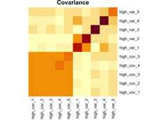
Now let’s make this dataset a little more complex. We can add afactor variable, some variables that discriminate between the levels ofthat factor, and add some missing values.
set.seed(501)df2<- df1%>%sim_cat(n_groups =3,name ="factor")%>%group_by(factor)%>%sim_discr(n_vars =5,var =1,cov =0,group_means =c(-1.3,0,1.3),name ="discr")%>%sim_discr(n_vars =5,var =1,cov =0,group_means =c(0,0.5,1),name ="discr2")%>%sim_missing(prop =0.1)%>%ungroup()df2#> # A tibble: 20 × 21#> factor high_cov_1 high_cov_2 high_cov_3 high_cov_4 high_cov_5 high_var_1#> <chr> <dbl> <dbl> <dbl> <dbl> <dbl> <dbl>#> 1 a 0.472 -0.362 0.253 0.281 NA -0.0873#> 2 a -1.50 -1.65 -1.47 -1.93 NA NA#> 3 a 1.13 NA NA 1.41 0.345 0.871#> 4 a 0.982 0.740 1.16 1.14 0.866 NA#> 5 a -0.773 NA NA -1.21 -1.25 -1.53#> 6 a 0.302 0.130 -0.309 0.0725 0.725 0.890#> 7 a -0.117 0.00163 0.0596 -0.542 -0.269 NA#> 8 b 2.16 2.47 1.38 1.62 1.62 -2.43#> 9 b NA -0.509 -0.529 -0.842 -1.04 1.25#> 10 b 0.609 0.195 0.720 0.930 0.595 -0.562#> 11 b 1.81 1.15 1.43 1.09 1.39 -0.934#> 12 b 0.954 0.234 0.247 0.248 0.751 1.95#> 13 b -1.03 NA -1.70 -1.27 -1.64 0.670#> 14 b NA 0.380 0.177 NA 0.550 2.68#> 15 c -0.214 -0.390 -0.476 -0.878 -0.328 0.665#> 16 c 0.827 0.556 0.620 0.491 0.814 -0.0121#> 17 c -0.399 -0.862 -0.385 -0.935 -0.802 NA#> 18 c -1.09 -1.32 -0.720 -1.88 -1.76 -2.05#> 19 c -0.181 -0.155 -0.774 0.0395 -0.770 1.81#> 20 c 0.882 NA 0.758 1.24 NA 1.11#> # ℹ 14 more variables: high_var_2 <dbl>, high_var_3 <dbl>, high_var_4 <dbl>,#> # high_var_5 <dbl>, discr_1 <dbl>, discr_2 <dbl>, discr_3 <dbl>,#> # discr_4 <dbl>, discr_5 <dbl>, discr2_1 <dbl>, discr2_2 <dbl>,#> # discr2_3 <dbl>, discr2_4 <dbl>, discr2_5 <dbl>pca<-opls(select(df2,-factor),fig.pdfC ="none",info.txtC ="none")plot(pca,parAsColFcVn = df2$factor,typeVc ="x-score")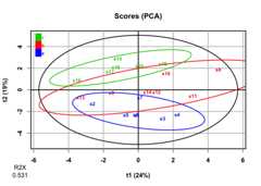
getLoadingMN(pca)%>%as_tibble(rownames ="variable")%>%arrange(desc(abs(p1)))#> # A tibble: 20 × 4#> variable p1 p2 p3#> <chr> <dbl> <dbl> <dbl>#> 1 high_cov_2 0.415 0.0534 0.0137#> 2 high_cov_1 0.407 0.0383 0.0208#> 3 high_cov_5 0.401 0.0163 0.104#> 4 high_cov_3 0.400 0.0301 -0.0837#> 5 high_cov_4 0.387 0.0218 0.00556#> 6 discr_5 -0.224 0.262 -0.136#> 7 high_var_2 -0.195 0.0848 0.240#> 8 discr2_1 0.167 0.396 -0.167#> 9 discr_2 -0.163 0.322 -0.202#> 10 high_var_5 0.115 -0.132 0.261#> 11 discr2_5 0.0967 0.267 0.114#> 12 high_var_1 -0.0930 -0.0102 0.457#> 13 discr2_4 0.0834 0.308 0.0924#> 14 discr_3 -0.0627 0.376 -0.0152#> 15 discr2_2 -0.0412 0.138 0.539#> 16 discr_1 -0.0407 0.319 0.0471#> 17 discr2_3 -0.0394 0.176 -0.358#> 18 discr_4 0.0363 0.400 0.144#> 19 high_var_3 -0.0101 -0.0629 0.0483#> 20 high_var_4 -0.00471 0.131 0.308It looks like PCA mostly picks up on the variables with highcovariance,not the variables that discriminate amonglevels offactor. This makes sense, as PCA is anunsupervised analysis.
plsda<-opls(select(df2,-factor), df2$factor,predI =2,permI =10,fig.pdfC ="none",info.txtC ="none")plot(plsda,typeVc ="x-score")
getVipVn(plsda)%>% tibble::enframe(name ="variable",value ="VIP")%>%arrange(desc(VIP))#> # A tibble: 20 × 2#> variable VIP#> <chr> <dbl>#> 1 discr_4 1.54#> 2 discr_1 1.48#> 3 discr_2 1.47#> 4 discr_5 1.44#> 5 discr_3 1.42#> 6 discr2_1 1.31#> 7 discr2_4 1.09#> 8 high_cov_2 1.08#> 9 discr2_3 0.996#> 10 high_cov_1 0.944#> 11 discr2_2 0.884#> 12 high_cov_5 0.790#> 13 discr2_5 0.650#> 14 high_var_5 0.639#> 15 high_var_2 0.582#> 16 high_cov_4 0.530#> 17 high_cov_3 0.423#> 18 high_var_4 0.358#> 19 high_var_1 0.200#> 20 high_var_3 0.0860PLS-DA, a supervised analysis, finds discrimination among groups andfinds that the discriminating variables we generated are mostresponsible for those differences.