Theordgam package enables to fit an additiveproportional odds model to ordinal data.
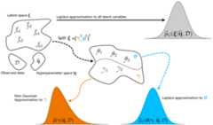
The combination ofLaplace approximations and ofBayesian P-splines (namedLPS) enable fast andflexible inference in a Bayesian framework. The Gaussian Markov randomfield prior assumed for the penalized spline parameters and theBernstein-von Mises theorem typically provide reliable Laplaceapproximation to the posterior distribution of these quantities.However, this accuracy can be seriously compromised for some unpenalizedparameters, especially when the information synthesized by the prior andthe likelihood is sparse.
We propose a refined version of the LPS methodology by splitting theparameter space in two subsets,
The marginal posterior density
Let us illustrate the use of theordgam package on a datasubset (\(n=552\)) from the EuropeanSocial Survey (ESS 2018) specific to the French speaking respondentsfrom Wallonia, one of the three regions in Belgium. Each of theparticipants (aged at least 15) was asked to react to the followingstatement,Gay men and lesbians should be free to live their ownlife as they wish, with a positioning on a Likert scale going from1 (Agree strongly) to 5 (Disagree strongly).
## Package installation and loading## install.packages("devtools")## devtools::install_github("plambertULiege/ordgam")library(ordgam)## Data readingdata(freehmsDataBE)donnees=subset(freehmsDataBE,region=="WAL")## Focus on Walloniahead(donnees)## freehms gndr age eduyrs region## 2 1 Male 25 17 WAL## 3 2 Female 76 6 WAL## 7 1 Male 69 17 WAL## 9 2 Male 36 10 WAL## 12 1 Male 54 7 WAL## 18 1 Female 28 14 WALLet us fit a proportional odds model to these data with the number ofcompleted years of education (\(14.1\pm4.4\) years) and age (\(47.3\pm18.5\) years) entering as additive terms,
## Model fit with a Gamma prior for the penalty parametersmod=ordgam(freehms~s(eduyrs)+s(age),data=donnees,descending =FALSE)print(mod)## Call:## ordgam(formula = freehms ~ s(eduyrs) + s(age), data = donnees, descending = FALSE) ## ## Prior set on the regression paramaters <beta>## ## Parameter estimation:## est se low up Z Pval ## 1 0.0272 0.1152 -0.1986 0.2530 0.24 0.81 ## 2 1.6318 0.1400 1.3574 1.9062 11.66 <2e-16 ***## 3 2.5509 0.1863 2.1858 2.9160 13.69 <2e-16 ***## 4 4.4168 0.4163 3.6008 5.2328 10.61 <2e-16 ***## ## Approximate significance of smooth terms:## edf Tr Pval Chi2 Pval ## f(eduyrs) 1.24 1.01 0.477617 1.15 0.35501 ## f(age) 2.55 18.77 0.000265 18.82 0.00017 ***## ## Selected penalty parameters <lambda>: 191.7967 18.40125 ## Lambda log prior: dgamma(lambda, 1, 1e-04, log = TRUE)## ## Likelihood - Information criterions (n = 552):## edf logL logLmarg AIC BIC ## 7.79 -598.66 -606.75 1212.90 1246.49 ## ## NOTE: model the odds of a response value in the lower scaleThe estimated additive terms can also be visualized:
plot(mod,mfrow=c(1,2))The asymmetry of the posterior for the non-penalized parameters
model= mod## Model for which the approximation is required## Skew-t approximation to the marginal of gamma.tilde[k]ngamma=with(model, nalpha+nfixed)## Number of non-penalized parmsgamt.ST=list()## Skew-t coefs --> dst(x,dp=coef)for (kin1:ngamma){## Loop over the gamma.tilde components x.grid=seq(-4,4,length=10)## Grid of values for gamma.tilde[k] lfy.grid= ordgam::lmarg.gammaTilde(x.grid,k=k,model)## log p(gamma.tilde[k] | D) gamt.ST[[k]]= ordgam:::STapprox(x.grid,lfy.grid)$dp## Approximate using a skew-t}## Visualization of the posterior for <gamma.tilde[k]>par(mfrow=c(2,2),mar=c(4,5,1,1))for (kin1:ngamma){## Loop over the gamma.tilde components xlab=bquote(tilde(gamma)[.(k)]) ylab=bquote(p(tilde(gamma)[.(k)]~"|"~lambda~","~D)) xlim= sn::qst(c(.0001,.9999),dp=gamt.ST[[k]])curve(sn::dst(x,dp=gamt.ST[[k]]),xlim=xlim,xlab=xlab,ylab=ylab,col="blue",lwd=2,lty=1)}
The results can be re-expressed in the original parametrization,yieding\(p(\gamma_k|\lambda,{\calD})\) and a noticable asymmetry for the posterior density of\(\gamma_4\):
## Sampling <gamma.tilde> using the (approximate) independence of its componentsM=10000sample.tilde=matrix(nrow=M,ncol=ngamma)for (kin1:ngamma){## ... or using skew-t approximation sample.tilde[,k]=c(sn::rst(M,dp=gamt.ST[[k]]))}## Revert sample to the original <gamma> parametrizationgam.hat= model$theta[1:ngamma]## MAP estimateSig= model$Sigma.theta[1:ngamma,1:ngamma]## Variance-covariancesv=svd(Sig) ; V= sv$u ; omega= sv$d## SVDsample.gam=t(gam.hat+ V%*% (sqrt(omega)*t(sample.tilde)))## Skew-t approximation to the marginal of gam[k]gam.ST= gam.ST2=list()for (kin1:ngamma){ temp=hist(sample.gam[,k],plot=FALSE) gam.ST[[k]]= ordgam:::STapprox(temp$mids,log(temp$density+1e-6))$dp## temp = selm(sample.gam[,k] ~ 1, family="ST")## gam.ST2[[k]] = coef(temp,"DP")}## Visualize p(gamma[k] | lambda,data)par(mfrow=c(2,2),mar=c(4,5,1,1))for (kin1:ngamma){ xlab=bquote(gamma[.(k)]) ylab=bquote(p(gamma[.(k)]~"|"~lambda~","~D)) xlim= sn::qst(c(.0001,.9999),dp=gam.ST[[k]])curve(sn::dst(x,dp=gam.ST[[k]]),lwd=2,col="blue",xlim=xlim,xlab=xlab,ylab=ylab)}
Let us revisit the same model for the data collected in Flanders, themost populated region of Belgium.
## Model fit with a Gamma prior for the penalty parametersmod.FL=ordgam(freehms~s(eduyrs)+s(age),data=subset(freehmsDataBE,region=="FL"),descending =FALSE)print(mod.FL)## Call:## ordgam(formula = freehms ~ s(eduyrs) + s(age), descending = FALSE,## data = subset(freehmsDataBE, region == "FL")) ## ## Prior set on the regression paramaters <beta>## ## Parameter estimation:## est se low up Z Pval ## 1 0.3176 0.0866 0.1479 0.4872 3.67 0.00024 ***## 2 2.7105 0.1367 2.4426 2.9784 19.83 < 2e-16 ***## 3 3.4898 0.1829 3.1312 3.8484 19.08 < 2e-16 ***## 4 4.8852 0.3407 4.2174 5.5530 14.34 < 2e-16 ***## ## Approximate significance of smooth terms:## edf Tr Pval Chi2 Pval ## f(eduyrs) 1.15 27.7 9.64e-07 29.0 1.0e-07 ***## f(age) 2.57 34.6 1.41e-06 34.6 7.9e-08 ***## ## Selected penalty parameters <lambda>: 296.6694 33.87409 ## Lambda log prior: dgamma(lambda, 1, 1e-04, log = TRUE)## ## Likelihood - Information criterions (n = 1046):## edf logL logLmarg AIC BIC ## 7.72 -923.13 -932.09 1861.70 1899.94 ## ## NOTE: model the odds of a response value in the lower scalefhat.FL=plot(mod.FL,mfrow=c(1,2))
The estimated additive terms for education and age look a bitdifferent from the estimates for Wallonia with, here, the suggestion ofa statistically significant and linear effect of ‘eduyrs’.
The marginal posterior distribution of the log of the penaltyparameters,\(\nu_j=\log\lambda_j\),can be visualized and compared to the their prior:
model= mod.FL## log(lambda) marginal posteriorspar(mfrow=c(1,2),mar=c(4,5,3,1))for (jin1:2){## Loop over <nu> components## Plot of the approximating skew-t to the marginal posterior of <nu[j]> xlims= sn::qst(c(.001,.999),dp=model$nu.dp[[j]]) xlab=bquote(log(lambda[.(j)])) ylab=bquote(p(log(lambda[.(j)])~"|"~D))curve(sn::dst(x,dp=model$nu.dp[[j]]),xlims[1],xlims[2],lwd=2,col="red",main=names(model$lambda)[j],xlab=xlab,ylab=ylab,ylim=c(0,.4))## ... compared to the prior for <nu[j]>curve(exp(model$lprior.lambda(exp(x)))*exp(x),add=T,lty=3,lwd=2)legend("topright",legend=c("Posterior","Prior"),lwd=c(2,2),lty=c(1,3),col=c("red","black"),horiz=TRUE,bty="n",cex=1)}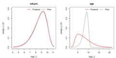
While the first posterior associated to penalty parameter for‘eduyrs’ does not depart from its prior with a large prior mean (as\(\lambda_1 \sim {\cal G}(1,10^{-4})\)has prior mean\(10^4\)) and suggestslinearity, the posterior associated to
ordgam: Additive proportional odds model for ordinaldata using Laplace approximations and Bayesian P-splines. Copyright (C)2022-2023 Philippe Lambert
This program is free software: you can redistribute it and/or modifyit under the terms of the GNU General Public License as published by theFree Software Foundation, either version 3 of the License, or (at youroption) any later version.
This program is distributed in the hope that it will be useful, butWITHOUT ANY WARRANTY; without even the implied warranty ofMERCHANTABILITY or FITNESS FOR A PARTICULAR PURPOSE. See the GNU GeneralPublic License for more details.
You should have received a copy of the GNU General Public Licensealong with this program. If not, seehttps://www.gnu.org/licenses/.
[1] Lambert, P. and Gressani, O (2023). Penalty parameter selectionand asymmetry corrections to Laplace approximations in BayesianP-splines models.Statistical Modellingdoi:10.1177/1471082X231181173.Preprint:arXiv:2210.01668
[2] Lambert, P. (2023) R-packageordgam - CRAN and GitHub:plambertULiege/ordgam