

The actxps package provides a set of tools to assist with thecreation of actuarial experience studies. Experience studies are used byactuaries to explore historical experience across blocks of business andto inform assumption setting for projection models.
expose() family of functions convert census-levelrecords into policy or calendar year exposure records.exp_stats() function creates experience summarydata frames containing observed termination rates and claims.Optionally, expected termination rates, actual-to-expected ratios, andlimited fluctuation credibility estimates can also be returned.add_transactions() function attaches summarizedtransactions to a data frame with exposure-level records.trx_stats() function creates transaction summarydata frames containing transaction counts, amounts, frequencies, andutilization. Optionally, transaction amounts can be expressed as apercentage of one or more variables to calculate rates oractual-to-expected ratios.autoplot() andautotable() functionscreates plots and tables for reporting.exp_shiny() function launches a Shiny app thatallows for interactive exploration of experience drivers.The actxps package can be installed from CRAN with:
install.packages("actxps")To install the development version fromGitHub use:
devtools::install_github("mattheaphy/actxps")An expanded version of this demo is available invignette("actxps").
The actxps package includes simulated census data for a theoreticaldeferred annuity product with an optional guaranteed income rider. Thegrain of this data is one rowper policy.
library(actxps)library(dplyr)census_dat#> # A tibble: 20,000 × 11#> pol_num status issue_date inc_guar qual age product gender wd_age premium#> <int> <fct> <date> <lgl> <lgl> <int> <fct> <fct> <int> <dbl>#> 1 1 Active 2014-12-17 TRUE FALSE 56 b F 77 370#> 2 2 Surren… 2007-09-24 FALSE FALSE 71 a F 71 708#> 3 3 Active 2012-10-06 FALSE TRUE 62 b F 63 466#> 4 4 Surren… 2005-06-27 TRUE TRUE 62 c M 62 485#> 5 5 Active 2019-11-22 FALSE FALSE 62 c F 67 978#> 6 6 Active 2018-09-01 FALSE TRUE 77 a F 77 1288#> 7 7 Active 2011-07-23 TRUE TRUE 63 a M 65 1046#> 8 8 Active 2005-11-08 TRUE TRUE 58 a M 58 1956#> 9 9 Active 2010-09-19 FALSE FALSE 53 c M 64 2165#> 10 10 Active 2012-05-25 TRUE FALSE 61 b M 73 609#> # ℹ 19,990 more rows#> # ℹ 1 more variable: term_date <date>Convert census records to exposure records with one rowperpolicy per year.
exposed_data<-expose(census_dat,end_date ="2019-12-31",target_status ="Surrender")exposed_data#>#> ── Exposure data ──#>#> • Exposure type: policy_year#> • Target status: Surrender#> • Study range: 1900-01-01 to 2019-12-31#>#> # A tibble: 141,252 × 15#> pol_num status issue_date inc_guar qual age product gender wd_age premium#> <int> <fct> <date> <lgl> <lgl> <int> <fct> <fct> <int> <dbl>#> 1 1 Active 2014-12-17 TRUE FALSE 56 b F 77 370#> 2 1 Active 2014-12-17 TRUE FALSE 56 b F 77 370#> 3 1 Active 2014-12-17 TRUE FALSE 56 b F 77 370#> 4 1 Active 2014-12-17 TRUE FALSE 56 b F 77 370#> 5 1 Active 2014-12-17 TRUE FALSE 56 b F 77 370#> 6 1 Active 2014-12-17 TRUE FALSE 56 b F 77 370#> 7 2 Active 2007-09-24 FALSE FALSE 71 a F 71 708#> 8 2 Active 2007-09-24 FALSE FALSE 71 a F 71 708#> 9 2 Active 2007-09-24 FALSE FALSE 71 a F 71 708#> 10 2 Active 2007-09-24 FALSE FALSE 71 a F 71 708#> # ℹ 141,242 more rows#> # ℹ 5 more variables: term_date <date>, pol_yr <int>, pol_date_yr <date>,#> # pol_date_yr_end <date>, exposure <dbl>Create a summary grouped by policy year and the presence of aguaranteed income rider.
exp_res<- exposed_data|>group_by(pol_yr, inc_guar)|>exp_stats()exp_res#>#> ── Experience study results ──#>#> • Groups: pol_yr and inc_guar#> • Target status: Surrender#> • Study range: 1900-01-01 to 2019-12-31#>#> # A tibble: 30 × 6#> pol_yr inc_guar n_claims claims exposure q_obs#> <int> <lgl> <int> <int> <dbl> <dbl>#> 1 1 FALSE 56 56 7720. 0.00725#> 2 1 TRUE 46 46 11532. 0.00399#> 3 2 FALSE 92 92 7103. 0.0130#> 4 2 TRUE 68 68 10612. 0.00641#> 5 3 FALSE 67 67 6447. 0.0104#> 6 3 TRUE 57 57 9650. 0.00591#> 7 4 FALSE 123 123 5799. 0.0212#> 8 4 TRUE 45 45 8737. 0.00515#> 9 5 FALSE 97 97 5106. 0.0190#> 10 5 TRUE 67 67 7810. 0.00858#> # ℹ 20 more rowsCalculate actual-to-expected ratios.
First, attach one or more columns of expected termination rates tothe exposure data. Then, pass these column names to theexpected argument ofexp_stats().
expected_table<-c(seq(0.005,0.03,length.out =10),0.2,0.15,rep(0.05,3))# using 2 different expected termination ratesexposed_data<- exposed_data|>mutate(expected_1 = expected_table[pol_yr],expected_2 =ifelse(exposed_data$inc_guar,0.015,0.03))exp_res<- exposed_data|>group_by(pol_yr, inc_guar)|>exp_stats(expected =c("expected_1","expected_2"))exp_res#>#> ── Experience study results ──#>#> • Groups: pol_yr and inc_guar#> • Target status: Surrender#> • Study range: 1900-01-01 to 2019-12-31#> • Expected values: expected_1 and expected_2#>#> # A tibble: 30 × 10#> pol_yr inc_guar n_claims claims exposure q_obs expected_1 expected_2#> <int> <lgl> <int> <int> <dbl> <dbl> <dbl> <dbl>#> 1 1 FALSE 56 56 7720. 0.00725 0.005 0.03#> 2 1 TRUE 46 46 11532. 0.00399 0.005 0.015#> 3 2 FALSE 92 92 7103. 0.0130 0.00778 0.03#> 4 2 TRUE 68 68 10612. 0.00641 0.00778 0.015#> 5 3 FALSE 67 67 6447. 0.0104 0.0106 0.03#> 6 3 TRUE 57 57 9650. 0.00591 0.0106 0.015#> 7 4 FALSE 123 123 5799. 0.0212 0.0133 0.03#> 8 4 TRUE 45 45 8737. 0.00515 0.0133 0.015#> 9 5 FALSE 97 97 5106. 0.0190 0.0161 0.03#> 10 5 TRUE 67 67 7810. 0.00858 0.0161 0.015#> # ℹ 20 more rows#> # ℹ 2 more variables: ae_expected_1 <dbl>, ae_expected_2 <dbl>Create visualizations using theautoplot() andautotable() functions.
autoplot(exp_res)
# first 10 rows showed for brevityexp_res|>head(10)|>autotable()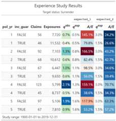
Launch a Shiny app to interactively explore experience data.
exp_shiny(exposed_data)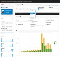
Logo
Imageby macrovector on Freepik