fit and compareSpecies-Area Relationship (SAR)models using multi-model inference
sars provides functionality to fit twenty SAR modelusing non-linear regression, and to calculate multi-model averagedcurves using various information criteria. The software also provideseasy to use functionality to plot multi-model SAR curves and to generateconfidence intervals using bootstrapping. Additional SAR relatedfunctions include fitting the linear version of the power model andcomparing parameters with the non-linear version, fitting the generaldynamic model of island biogeography, fitting the random placement modelto a species abundance-site matrix, and extrapolating fitted SAR modelsto predict richness on larger islands / sample areas. Version 1.3.0 hasadded functions for fitting, evaluating and plotting a range of commonlyused piecewise SAR models (see Matthews and Rigal (2021) for details onthese functions). Version 2.0.0 has added functions to fit a range ofhabitat and countryside SAR models (see Furness et al. (2023), Pereiraand Daily (2006) and Proenca and Pereira (2013)), along with associatedplot and prediction functions.
Please report any bugs or issues to us via GitHub.
The package has an associated vignette that provides examples of howto use the package, and three accompanying papers (Matthews etal. (2019), Matthews and Rigal (2021) and Matthews et al. (2025) Inreview).
Version 1.1.1 of the package has been archived on the Zenodo researchdata repository (DOI: 10.5281/zenodo.2573067).
You can install the released version of sars fromCRAN with:
install.packages("sars")And the development version fromGitHub with:
# install.packages("devtools")devtools::install_github("txm676/sars")Basic usage ofsars will result in using two typesof functions:
To fit the power sar model (Arrhenius 1921) to the ‘galapagos’(Preston 1962) data set:
fit_pow<-sar_power(data = galap)fit_pow#>#> Model:#> Power#>#> Call:#> S == c * A^z#>#> Coefficients:#> c z#> 33.1791553 0.2831868Attempting to fit all 20 sar models to the ‘galapagos’ (Preston 1962)data set and get a multi-model SAR:
mm_galap<-sar_average(data = galap)#>#> Models to be fitted using a grid start approach:#>#> Now attempting to fit the 20 SAR models:#>#> ── multi_sars ────────────────────────────────────────────── multi-model SAR ──#> → power : ✔#> → powerR : ✔#> → epm1 : ✔#> → epm2 : ✔#> → p1 : ✔#> → p2 : ✔#> → loga : ✔#> → koba : ✔#> → monod : ✔#> → negexpo : ✔#> → chapman : ✔#> → weibull3 : ✔#> → asymp : ✔#> → ratio : ✔#> → gompertz : ✔#> → weibull4 : ✔#> → betap : ✔#> → logistic : ✔#> → heleg : ✔#> → linear : ✔#>#> No model validation checks selected#>#> 20 remaining models used to construct the multi SAR:#> Power, PowerR, Extended Power model 1, Extended Power model 2, Persistence function 1, Persistence function 2, Logarithmic, Kobayashi, Monod, Negative exponential, Chapman Richards, Cumulative Weibull 3 par., Asymptotic regression, Rational function, Gompertz, Cumulative Weibull 4 par., Beta-P cumulative, Logistic(Standard), Heleg(Logistic), Linear model#> ────────────────────────────────────────────────────────────────────────────────Each of the ‘fitted’ objects have corresponding plot methods:
To fit the logarithmic SAR model (Gleason 1922) to the ‘galapagos’data set and plot it
fit_loga<-sar_loga(data = galap)plot(fit_loga)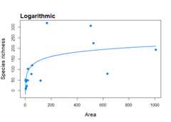
To fit a multimodel SAR curve to the ‘galapagos’ data set and plot it(alongside the individual model fits)
mm_galap<-suppressMessages(sar_average(data = galap,verb =FALSE))#>#> Models to be fitted using a grid start approach:#>#> Now attempting to fit the 20 SAR models:#>#> ── multi_sars ────────────────────────────────────────────── multi-model SAR ──#> → power : ✔#> → powerR : ✔#> → epm1 : ✔#> → epm2 : ✔#> → p1 : ✔#> → p2 : ✔#> → loga : ✔#> → koba : ✔#> → monod : ✔#> → negexpo : ✔#> → chapman : ✔#> → weibull3 : ✔#> → asymp : ✔#> → ratio : ✔#> → gompertz : ✔#> → weibull4 : ✔#> → betap : ✔#> → logistic : ✔#> → heleg : ✔#> → linear : ✔#>#> No model validation checks selected#>#> 20 remaining models used to construct the multi SAR:#> Power, PowerR, Extended Power model 1, Extended Power model 2, Persistence function 1, Persistence function 2, Logarithmic, Kobayashi, Monod, Negative exponential, Chapman Richards, Cumulative Weibull 3 par., Asymptotic regression, Rational function, Gompertz, Cumulative Weibull 4 par., Beta-P cumulative, Logistic(Standard), Heleg(Logistic), Linear model#> ────────────────────────────────────────────────────────────────────────────────mm_galap#>#> This is a sar_average fit object:#>#> 20 models successfully fitted#>#> AICc used to rank modelsplot(mm_galap,pLeg =FALSE,mmSep =TRUE)
To fit the two-threshold continuous model to the ‘aegean2’dataset
fit<-sar_threshold(data = aegean2,mod =c("ContTwo"),interval =0.1,non_th_models =FALSE,logAxes ="area",con =1,logT = log10,nisl =NULL)plot(fit,cex =0.8,cex.main =1.1,cex.lab =1.1,pcol ="grey")
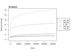
To fit the countryside SAR model (power form) to the ‘countryside’dataset and generate one of a range of different plots of the model fitthat can be generated
s3<-sar_countryside(data = countryside,modType ="power",gridStart ="none",habNam =c("AG","SH","F"),spNam =c("AG_Sp","SH_Sp","F_Sp","UB_Sp"))par(mar=c(5.1,4.1,4.1,7.5),xpd=TRUE)plot(s3,type =2,totSp =TRUE,lcol =c("black","aquamarine4","#CC661AB3" ,"darkblue","darkgrey"),pLeg =TRUE,legPos ="topright",legInset =c(-0.27,0.3),lwd =1.5,ModTitle =c("Agricultural land","Shrubland","Forest"),which =2)