


Overview
Thevecmatch package implements the Vector Matchingalgorithm introduced in the paperEstimation of Causal Effects withMultiple Treatments: A Review and New Ideas by Lopez and Gutman(2017). This package allows users to:
- Visualize initial covariate imbalances with elegant graphics.
- Estimate treatment assignment probabilities using various regressionmodels.
- Define the common support region.
- Perform matching across multiple treatment groups.
- Evaluate the quality of matching.
Installation
You can install the latest version ofvecmatch fromGitHub with:
# Install devtools if its not already installedif(!require(devtools)){install.packages("devtools")library(devtools)}# Install the vecmatch package directly from githubdevtools::install_github("Polymerase3/vecmatch")Once the package is released on CRAN, you can install it using thestandard workflow:install.packages("vecmatch").
vecmatch Workflow
The vecmatch package has an exact workflow and it is advisable tofollow it. It consists of 5 steps and ensures the best possible matchingquality using the vector matching algorithm:
1. Initial imbalanceassessment
Visualize covariate imbalances in your dataset using theraincloud() function for continuous variables and themosaic() function for categorical variables. Both functionssupport grouping by up to two categorical variables (groupandfacet arguments) and provide standardized meandifferences and significance tests.
library(vecmatch)raincloud(data = cancer,y = bmi,group = status,facet = sex,significance ="t_test",sig_label_color =TRUE,sig_label_size =3,limits =c(7,48))#> Warning: Removed 9 rows containing missing values or values outside the scale range#> (`geom_flat_violin()`).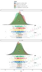
2. EstimateGeneralized Propensity Scores (GPS)
Next, estimate generalized propensity scores for the treatmentvariable. These scores represent treatment assignment probabilitiesbased on user-defined covariates. Use theestimate_gps()function to estimate GPS. As a result, a matrix of generalizedpropensity scores is returned:
formula_cancer<-formula(status~ bmi* sex)gps_matrix<-estimate_gps(formula_cancer,data = cancer,method ="vglm",reference ="control")head(gps_matrix,n =7)#> gps object (generalized propensity scores)#> • Number of units: 7#> • Number of treatments: 4#> • Treatment column: treatment#> • GPS probability columns: control, adenoma, crc_benign, crc_malignant#> • Treatment levels: control, adenoma, crc_benign, crc_malignant#> • All columns except 'treatment' store probabilities in [0, 1].#>#> treatment control adenoma crc_benign crc_malignant#> 1 control 0.3347396 0.2858184 0.1622951 0.2171469#> 2 control 0.2397453 0.3487326 0.2006854 0.2108367#> 3 control 0.2400506 0.2885477 0.2533414 0.2180602#> 4 control 0.2478800 0.2856531 0.2783953 0.1880716#> 5 control 0.2398759 0.2848793 0.2568960 0.2183489#> 6 control 0.2652354 0.2878765 0.2518512 0.1950369#> 7 control 0.2806189 0.2888866 0.2297684 0.2007260As you can see, each row in the resulting GPS matrix containstreatment assignment probabilities for all levels of the treatmentvariable, summing to 1.
3. Define the CommonSupport Region (CSR)
The next step involves estimating the boundaries of the commonsupport region (CSR). The lower and upper CSR boundaries define therange of propensity scores where observations are present across alltreatment groups. You can calculate these boundaries by applying thecsregion() function to thegps_matrixobject:
csr_matrix<-csregion(gps_matrix)Thecsregion() function outputs a matrix of generalizedpropensity scores, excluding any observations that fall outside the CSR.Additionally, it provides a summary of the process in the console. Youcan retrieve additional attributes of the csr_matrix object using theattr() function. Details about these attributes can befound in the documentation forcsregion().
4. Matchingon the Generalized Propensity Scores
You can use thecsr_matrix object to perform the actualmatching with the vector matching algorithm using thematch_gps() function. In this example, matching isperformed without replacement, using a larger caliper and a one-to-onematching ratio:
matched_data<-match_gps(csmatrix = csr_matrix,reference ="control",caliper =1)5. Assessing MatchingQuality
Finally, the quality of the matching process can be evaluated usingthebalqual() function. This function provides both meanand maximum values for various metrics, such as the standardized meandifference, variance ratio, and r-effect size coefficient.
balqual(matched_data, formula_cancer,statistic ="max")#>#> Matching Quality Evaluation#> ================================================================================#>#> Count table for the treatment variable:#> --------------------------------------------------#> Treatment | Before | After#> --------------------------------------------------#> adenoma | 355 | 148#> control | 304 | 148#> crc_benign | 279 | 148#> crc_malignant | 249 | 148#> --------------------------------------------------#>#>#> Matching summary statistics:#> ----------------------------------------#> Total n before matching: 1187#> Total n after matching: 592#> % of matched observations: 49.87 %#> Total maximal SMD value: 0.041#> Total maximal r value: 0.003#> Total maximal Var value: 1.009#>#>#> Maximal values :#> --------------------------------------------------------------------------------#> Variable | Coef | Before | After | Quality#> --------------------------------------------------------------------------------#> bmi | SMD | 0.245 | 0.041 | Balanced#> bmi | r | 0.010 | 0.003 | Balanced#> bmi | Var | 1.101 | 1.009 | Balanced#> sexF | SMD | 0.153 | 0.000 | Balanced#> sexF | r | 0.006 | 0.000 | Balanced#> sexF | Var | 1.004 | 1.000 | Balanced#> sexM | SMD | 0.153 | 0.000 | Balanced#> sexM | r | 0.006 | 0.000 | Balanced#> sexM | Var | 1.004 | 1.000 | Balanced#> bmi:sexF | SMD | 0.152 | 0.004 | Balanced#> bmi:sexF | r | 0.007 | 0.001 | Balanced#> bmi:sexF | Var | 1.042 | 1.004 | Balanced#> bmi:sexM | SMD | 0.151 | 0.006 | Balanced#> bmi:sexM | r | 0.006 | 0.001 | Balanced#> bmi:sexM | Var | 1.023 | 1.006 | Balanced#> --------------------------------------------------------------------------------Help
You can open the full documentation of the vecmatch packageusing:
help(package = vecmatch)[8]ページ先頭