![]()

‘corx’ aims to be a Swiss Army knife for correlation matrices.Formatting correlation matrices for academic tables can be challenging.‘corx’ does all the heavy lifting for you. It runs the correlations, andstores all relevant results in a list. Results can be formatted intodata.frames which can then easily be rendered into tables in a varietyof formats.
You can install the released version of corx fromCRAN with:
install.packages("corx")To try features in development, you can install corx from github
remotes::install_github("conig/corx@devel")The simplest way to use corx is to supply it with a data.frame, whichhouses numeric variables.
library(corx)x<-corx(mtcars)x#> corx(data = mtcars)#>#> ----------------------------------------------------------------------------#> mpg cyl disp hp drat wt qsec vs am#> ----------------------------------------------------------------------------#> mpg - -.85*** -.85*** -.78*** .68*** -.87*** .42* .66*** .60***#> cyl -.85*** - .90*** .83*** -.70*** .78*** -.59*** -.81*** -.52**#> disp -.85*** .90*** - .79*** -.71*** .89*** -.43* -.71*** -.59***#> hp -.78*** .83*** .79*** - -.45** .66*** -.71*** -.72*** -.24#> drat .68*** -.70*** -.71*** -.45** - -.71*** .09 .44* .71***#> wt -.87*** .78*** .89*** .66*** -.71*** - -.17 -.55*** -.69***#> qsec .42* -.59*** -.43* -.71*** .09 -.17 - .74*** -.23#> vs .66*** -.81*** -.71*** -.72*** .44* -.55*** .74*** - .17#> am .60*** -.52** -.59*** -.24 .71*** -.69*** -.23 .17 -#> gear .48** -.49** -.56*** -.13 .70*** -.58*** -.21 .21 .79***#> carb -.55** .53** .39* .75*** -.09 .43* -.66*** -.57*** .06#> gear carb#> mpg .48** -.55**#> cyl -.49** .53**#> disp -.56*** .39*#> hp -.13 .75***#> drat .70*** -.09#> wt -.58*** .43*#> qsec -.21 -.66***#> vs .21 -.57***#> am .79*** .06#> gear - .27#> carb .27 -#> ----------------------------------------------------------------------------#> Note. * p < 0.05; ** p < 0.01; *** p < 0.001To calculate correlations controlling for other variables, use the‘z’ argument.
x<-corx(mtcars,z = wt,caption ="Correlations controlling for weight")x#> corx(data = mtcars, z = wt, caption = "Correlations controlling for weight")#>#> Correlations controlling for weight#> -------------------------------------------------------------------------------#> mpg cyl disp hp drat qsec vs am gear carb#> -------------------------------------------------------------------------------#> mpg - -.56** -.34 -.55** .18 .55** .44* .00 -.06 -.40*#> cyl -.56** - .72*** .68*** -.33 -.74*** -.73*** .04 -.07 .34#> disp -.34 .72*** - .60*** -.24 -.62*** -.57*** .07 -.10 .04#> hp -.55** .68*** .60*** - .04 -.80*** -.57*** .39* .42* .69***#> drat .18 -.33 -.24 .04 - -.05 .08 .43* .50** .34#> qsec .55** -.74*** -.62*** -.80*** -.05 - .79*** -.49** -.39* -.65***#> vs .44* -.73*** -.57*** -.57*** .08 .79*** - -.36* -.17 -.44*#> am .00 .04 .07 .39* .43* -.49** -.36* - .67*** .54**#> gear -.06 -.07 -.10 .42* .50** -.39* -.17 .67*** - .71***#> carb -.40* .34 .04 .69*** .34 -.65*** -.44* .54** .71*** -#> -------------------------------------------------------------------------------#> Note. * p < 0.05; ** p < 0.01; *** p < 0.001Sometimes you only want the relationships for a subset of variables.Asymmetric matrices are useful in these instances. The arguments ‘x’ and‘y’ can be used to achieve this. ‘x’ sets row variables, ‘y’ sets columnvariables.
x<-corx(mtcars,x =c(mpg, wt))x#> corx(data = mtcars, x = c(mpg, wt))#>#> -------------------#> mpg wt#> -------------------#> mpg - -.87***#> wt -.87*** -#> -------------------#> Note. * p < 0.05; ** p < 0.01; *** p < 0.001x<-corx(mtcars,x =c(mpg, wt),y =c(hp, gear, am))x#> corx(data = mtcars, x = c(mpg, wt), y = c(hp, gear, am))#>#> ---------------------------#> hp gear am#> ---------------------------#> mpg -.78*** .48** .60***#> wt .66*** -.58*** -.69***#> ---------------------------#> Note. * p < 0.05; ** p < 0.01; *** p < 0.001Users can further customise the table for publication. For instance,the numbers of significance stars can be changed, the area above thediagonal omitted, and captions and notes added.
x<-corx(mtcars[,1:5],stars =c(0.05),triangle ="lower",caption ="An example correlation matrix")x#> corx(data = mtcars[, 1:5], stars = c(0.05), triangle = "lower",#> caption = "An example correlation matrix")#>#> An example correlation matrix#> -------------------------------#> 1 2 3 4#> -------------------------------#> 1. mpg -#> 2. cyl -.85* -#> 3. disp -.85* .90* -#> 4. hp -.78* .83* .79* -#> 5. drat .68* -.70* -.71* -.45*#> -------------------------------#> Note. * p < 0.05We can also add in descriptive statistics easily.
x<-corx(mtcars[,1:5],stars =c(0.05,0.01,0.001),triangle ="lower",caption ="An example correlation matrix",describe =c(M = mean,SD = sd, kurtosis))x#> corx(data = mtcars[, 1:5], stars = c(0.05, 0.01, 0.001), triangle = "lower",#> caption = "An example correlation matrix", describe = c(M = mean,#> SD = sd, kurtosis))#>#> An example correlation matrix#> -------------------------------------------------------------#> 1 2 3 4 M SD kurtosis#> -------------------------------------------------------------#> 1. mpg - 20.09 6.03 2.80#> 2. cyl -.85*** - 6.19 1.79 1.32#> 3. disp -.85*** .90*** - 230.72 123.94 1.91#> 4. hp -.78*** .83*** .79*** - 146.69 68.56 3.05#> 5. drat .68*** -.70*** -.71*** -.45** 3.60 0.53 2.44#> -------------------------------------------------------------#> Note. * p < 0.05; ** p < 0.01; *** p < 0.001To add descriptive columns describe can be set to any combination ofthe following values:c(“mean”,“sd”,“median”,“iqr”,“var”,“skewness”,“kurtosis”).
Alternatively, you can pass a list of named functions:
x<-corx(mtcars[,1:8],describe =list(Mean =function(x)mean(x),SD =function(x)sd(x)))x#> corx(data = mtcars[, 1:8], describe = list(Mean = function(x) mean(x),#> SD = function(x) sd(x)))#>#> ---------------------------------------------------------------------------#> mpg cyl disp hp drat wt qsec vs Mean#> ---------------------------------------------------------------------------#> mpg - -.85*** -.85*** -.78*** .68*** -.87*** .42* .66*** 20.09#> cyl -.85*** - .90*** .83*** -.70*** .78*** -.59*** -.81*** 6.19#> disp -.85*** .90*** - .79*** -.71*** .89*** -.43* -.71*** 230.72#> hp -.78*** .83*** .79*** - -.45** .66*** -.71*** -.72*** 146.69#> drat .68*** -.70*** -.71*** -.45** - -.71*** .09 .44* 3.60#> wt -.87*** .78*** .89*** .66*** -.71*** - -.17 -.55*** 3.22#> qsec .42* -.59*** -.43* -.71*** .09 -.17 - .74*** 17.85#> vs .66*** -.81*** -.71*** -.72*** .44* -.55*** .74*** - 0.44#> SD#> mpg 6.03#> cyl 1.79#> disp 123.94#> hp 68.56#> drat 0.53#> wt 0.98#> qsec 1.79#> vs 0.50#> ---------------------------------------------------------------------------#> Note. * p < 0.05; ** p < 0.01; *** p < 0.001Corx objects can be passed directly to papaja::apa_table(), orknitr::kable().
corx(mtcars[,1:5],triangle ="lower",describe =c(mean, sd))|> knitr::kable(caption ="My correlation matrix")| 1 | 2 | 3 | 4 | mean | sd | |
|---|---|---|---|---|---|---|
| 1. mpg | - | 20.09 | 6.03 | |||
| 2. cyl | -.85*** | - | 6.19 | 1.79 | ||
| 3. disp | -.85*** | .90*** | - | 230.72 | 123.94 | |
| 4. hp | -.78*** | .83*** | .79*** | - | 146.69 | 68.56 |
| 5. drat | .68*** | -.70*** | -.71*** | -.45** | 3.60 | 0.53 |
My correlation matrix
There are many useful functions for plotting correlation matrices.‘corx’ contains a plot function which uses the ‘ggcorrplot’ package.
plot(x)
Multidimensional scaling enables similarities between variables to beconverted to 2D distances. This lets us visualise how variables clustertogether.
plot_mds(x)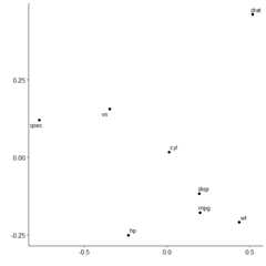
We can see that variables in mtcars cluster together in two separategroups. If we want to highlight this we can request two clusters to bemarked.
plot_mds(x,2)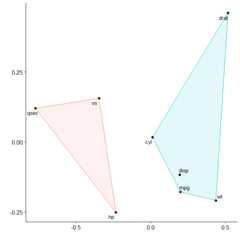
You can see that miles per gallon, the number of cylinders, thedisplacement rate, and the weight of the car are all closelyrelated.