Movatterモバイル変換

RevisitingWhittaker-Henderson Smoothing

What isWhittaker-Henderson smoothing ?

Origin

Whittaker-Henderson (WH) smoothing is a graduation method designed tomitigate the effects of sampling fluctuations in a vector of evenlyspaced discrete observations. Although this method was originallyproposed by Bohlmann (1899), it is named after Whittaker (1923), whoapplied it to graduate mortality tables, and Henderson (1924), whopopularized it among actuaries in the United States. The method waslater extended to two dimensions by Knorr (1984). WH smoothing may beused to build experience tables for a broad spectrum of life insurancerisks, such as mortality, disability, long-term care, lapse, mortgagedefault and unemployment.

The one-dimensional case

Let\(\mathbf{y}\) be a vector ofobservations and\(\mathbf{w}\) avector of positive weights, both of size\(n\). The estimator associated withWhittaker-Henderson smoothing is given by:

\[\hat{\mathbf{y}} =\underset{\boldsymbol{\theta}}{\text{argmin}}\{F(\mathbf{y},\mathbf{w},\boldsymbol{\theta})+ R_{\lambda,q}(\boldsymbol{\theta})\}\]

where:

• \(F(\mathbf{y},\mathbf{w},\boldsymbol{\theta}) =\underset{i = 1}{\overset{n}{\sum}} w_i(y_i - \theta_i)^2\)represents a fidelity criterion with respect to theobservations,

• \(R_{\lambda,q}(\boldsymbol{\theta}) =\lambda \underset{i = 1}{\overset{n - q}{\sum}}(\Delta^q\boldsymbol{\theta})_i^2\) represents a smoothnesscriterion.

In the latter expression,\(\lambda \ge0\) is a smoothing parameter and\(\Delta^q\) denotes the forward differenceoperator of order\(q\), such that forany\(i\in\{1,\dots,n - q\}\):

\[(\Delta^q\boldsymbol{\theta})_i = \underset{k = 0}{\overset{q}{\sum}}\begin{pmatrix}q \\ k\end{pmatrix}(- 1)^{q - k} \theta_{i + k}.\]

Define\(W =\text{Diag}(\mathbf{w})\), the diagonal matrix of weights, and\(D_{n,q}\) as the order\(q\) difference matrix of dimensions\((n-q) \times n\), such that\((D_{n,q}\boldsymbol{\theta})_i =(\Delta^q\boldsymbol{\theta})_i\) for all\(i \in [1, n-q]\). The first- andsecond-order difference matrices are given by:

\[D_{n,1} = \begin{bmatrix}-1 & 1 & 0 & \ldots & 0 \\0 & -1 & 1 & \ldots & 0 \\\vdots & \vdots & \vdots & \ddots & \vdots \\0 & \ldots & 0 & -1 & 1 \\\end{bmatrix}\quad\text{and}\quadD_{n,2} = \begin{bmatrix}1 & -2 & 1 & 0 & \ldots & 0 \\0 & 1 & -2 & 1 & \ldots & 0 \\\vdots & \vdots & \vdots & \vdots & \ddots & \vdots\\0 & \ldots & 0 & 1 & -2 & 1 \\\end{bmatrix}.\]

while higher-order difference matrices follow the recursive formula\(D_{n,q} = D_{n - 1,q - 1}D_{n,1}\).The fidelity and smoothness criteria can be rewritten with matrixnotations as:

\[F(\mathbf{y},\mathbf{w},\boldsymbol{\theta}) = (\mathbf{y} -\boldsymbol{\theta})^TW(\mathbf{y} - \boldsymbol{\theta}) \quad\text{and} \quad R_{\lambda,q}(\boldsymbol{\theta}) =\lambda\boldsymbol{\theta}^TD_{n,q}^TD_{n,q}\boldsymbol{\theta}\]

and the WH smoothing estimator thus becomes:

\[\hat{\mathbf{y}} = \underset{\boldsymbol{\theta}}{\text{argmin}}\left\lbrace(\mathbf{y} - \boldsymbol{\theta})^TW(\mathbf{y} -\boldsymbol{\theta}) +\boldsymbol{\theta}^TP_{\lambda}\boldsymbol{\theta}\right\rbrace\]

where\(P_{\lambda} = \lambdaD_{n,q}^TD_{n,q}\).

The two-dimensional case

In the two-dimensional case, consider a matrix\(Y\) of observations and a matrix\(\Omega\) of non-negative weights, both ofdimensions\(n_x \times n_z\). The WHsmoothing estimator solves:

\[\widehat{Y} = \underset{\Theta}{\text{argmin}}\{F(Y,\Omega, \Theta) +R_{\lambda,q}(\Theta)\}\]

where:

• \(F(Y,\Omega, \Theta) = \sum_{i =1}^{n_x}\sum_{j = 1}^{n_z} \Omega_{i,j}(Y_{i,j} -\Theta_{i,j})^2\) represents a fidelity criterion with respect tothe observations,

• \(R_{\lambda,q}(\Theta) = \lambda_x\sum_{j = 1}^{n_z}\sum_{i = 1}^{n_x - q_x}(\Delta^{q_x}\Theta_{\bullet,j})_i^2 + \lambda_z \sum_{i =1}^{n_x}\sum_{j = 1}^{n_z - q_z}(\Delta^{q_z}\Theta_{i,\bullet})_j^2\) is a smoothness criterionwith\(\lambda =(\lambda_x,\lambda_z)\).

This latter criterion adds row-wise and column regularizationcriteria to\(\Theta\), with respectiveorders\(q_x\) and\(q_z\), weighted by non-negative smoothingparameters\(\lambda_x\) and\(\lambda_z\). In matrix notation, let\(\mathbf{y} = \textbf{vec}(Y)\),\(\mathbf{w} = \textbf{vec}(\Omega)\), and\(\boldsymbol{\theta} =\textbf{vec}(\Theta)\) as the vectors obtained by stacking thecolumns of the matrices\(Y\),\(\Omega\), and\(\Theta\), respectively. Additionally,denote\(W = \text{Diag}(\mathbf{w})\)and\(n = n_x \times n_z\). Thefidelity and smoothness criteria become:

\[\begin{aligned}F(\mathbf{y},\mathbf{w}, \boldsymbol{\theta}) &= (\mathbf{y} -\boldsymbol{\theta})^TW(\mathbf{y} - \boldsymbol{\theta}) \\R_{\lambda,q}(\boldsymbol{\theta}) &=\boldsymbol{\theta}^{T}(\lambda_x I_{n_z} \otimesD_{n_x,q_x}^{T}D_{n_x,q_x} + \lambda_z D_{n_z,q_z}^{T}D_{n_z,q_z}\otimes I_{n_x}) \boldsymbol{\theta}.\end{aligned}\]

and the associated estimator takes the same form as in theone-dimensional case except

\[P_{\lambda} = \lambda_x I_{n_z} \otimesD_{n_x,q_x}^{T}D_{n_x,q_x} + \lambda_z D_{n_z,q_z}^{T}D_{n_z,q_z}\otimes I_{n_x}.\]

An explicit solution

If\(W + P_{\lambda}\) isinvertible, the WH smoothing equation admits the closed-formsolution:

\[\hat{\mathbf{y}} = (W +P_{\lambda})^{-1}W\mathbf{y}.\]

Indeed, as a minimum,\(\hat{\mathbf{y}}\) satisfies:

\[0 = \left.\frac{\partial}{\partial\boldsymbol{\theta}}\right|_{\hat{\mathbf{y}}}\left\lbrace(\mathbf{y} -\boldsymbol{\theta})^{T}W(\mathbf{y} - \boldsymbol{\theta}) +\boldsymbol{\theta}^{T}P_{\lambda}\boldsymbol{\theta}\right\rbrace = - 2W(y - \hat{\mathbf{y}}) +2P_{\lambda} \hat{\mathbf{y}}.\]

It follows that\((W +P_{\lambda})\hat{\mathbf{y}} = W\mathbf{y}\), proving the aboveresult. If\(\lambda \neq 0\),\(W + P_{\lambda}\) is invertible as long as\(\mathbf{w}\) has\(q\) non-zero elements in theone-dimensional case, and\(\Omega\)has at least\(q_x \times q_z\)non-zero elements spread across\(q_x\)different rows and\(q_z\) differentcolumns in the two-dimensional case. These conditions are always met inreal datasets.

How to use the package?

TheWH package features a unique main functionWH. Two arguments are mandatory for this function:

• The vector (or matrix in the two-dimension case)dcorresponding to the number of observed events of interest by age (or byage and duration in the two-dimension case).d should havenamed elements (or rows and columns) for the model results to beextrapolated.

• The vector (or matrix in the two-dimension case)eccorresponding to the portfolio central exposure by age (or by age andduration in the two-dimension case) whose dimensions should match thoseofd. The contribution of each individual to the portfoliocentral exposure corresponds to the time the individual was actuallyobserved with corresponding age (and duration in the two-dimensioncase). It always ranges from 0 to 1 and is affected by individualsleaving the portfolio, no matter the cause, as well as censoring andtruncating phenomena.

Additional arguments may be supplied, whose description is given inthe documentation of the functions.

The package also embed two fictive agregated datasets to illustratehow to use it:

• portfolio_mortality contains the agregated number ofdeaths and associated central exposure by age for an annuityportfolio.

• portfolio_LTC contains the agregated number ofdeaths and associated central exposure by age and duration (in years)since the onset of LTC for the annuitant database of a long-term careportfolio.

# One-dimensional caseWH_1d_fit<-WH(portfolio_mort$d, portfolio_mort$ec)Outer procedure completedin14 iterations, smoothing parameters:9327, final LAML:32.1

# Two-dimensional caseWH_2d_fit<-WH(portfolio_LTC$d, portfolio_LTC$ec)Outer procedure completedin63 iterations, smoothing parameters:1211.41,1.09, final LAML:276

FunctionWH outputs objects of class"WH_1d" and"WH_2d" to which additionalfunctions (including generic S3 methods) may be applied:

• Theprint function provides a glimpse of the fittedresults

WH_1d_fitAn object fitted using the WHfunctionInitial data contains45 data points:  Observation positions:50  to94Smoothing parameter selected:9327Associated degrees of freedom:6.8WH_2d_fitAn object fitted using the WHfunctionInitial data contains450 data points:  First dimension:70  to99  Second dimension:0  to14Smoothing parameters selected:1211.41.1Associated degrees of freedom:47

• Theplot function generates rough plots of the modelfit, the associated standard deviation, the model residuals or theassociated degrees of freedom. See theplot.WH_1d andplot.WH_2d functions help for more details.

plot(WH_1d_fit)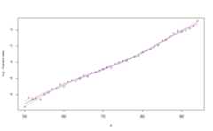

plot(WH_1d_fit,"res")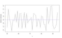

plot(WH_1d_fit,"edf")

plot(WH_2d_fit)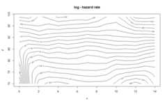

plot(WH_2d_fit,"std_y_hat")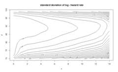

• Thepredict function generates an extrapolation of themodel. It requires anewdata argument, a named list withone or two elements corresponding to the positions of the newobservations. In the two-dimension case constraints are used so that thepredicted values matches the fitted values for the initial observations(see Carballo, Durban, and Lee 2021 to understand why this isrequired).

WH_1d_fit|>predict(newdata =40:99)|>plot()

WH_2d_fit|>predict(newdata =list(age =60:109,duration =0:19))|>plot()

• Thevcov may be used to retrieve thevariance-covariance matrix of the model if necessary.

• Finally theoutput_to_df function converts an"WH_1d" or"WH_2d" object into adata.frame. Information about the fit is discarded in theprocess. This function may be useful to produce better visualizationsfrom the data, for example using the ggplot2 package.

WH_1d_df<- WH_1d_fit|>output_to_df()WH_2d_df<- WH_2d_fit|>output_to_df()

Further WH smoothing theory

See the upcoming paper availablehere

References