

Efficient procedures for constrained likelihood estimation withtruncated lasso penalty (Shen et al., 2010; Zhang 2010) for linear andgeneralized linear models.
Note: this is a repo for the version published onCRAN. Please checkchunlinli/glmtlp for newfeatures such as constrained likelihood inference, regression on summarydata, memory efficiency, Gaussian graphical models, and more.
Installation
You can install the released version of glmtlp fromCRAN with:
install.packages("glmtlp")Examples for GaussianRegression Models
The following are three examples which show you how to useglmtlp to fit gaussian regression models:
library(glmtlp)data("gau_data")colnames(gau_data$X)[gau_data$beta!=0]#> [1] "V1" "V6" "V10" "V15" "V20"# Cross-Validation using TLP penaltycv.fit<-cv.glmtlp(gau_data$X, gau_data$y,family ="gaussian",penalty ="tlp",ncores=2)coef(cv.fit)[abs(coef(cv.fit))>0]#> intercept V1 V6 V10 V15 V20#> -0.009678041 1.240223517 0.883202180 0.725708239 1.125994003 0.981402236plot(cv.fit)
# Single Model Fit using TLP penaltyfit<-glmtlp(gau_data$X, gau_data$y,family ="gaussian",penalty ="tlp")coef(fit,lambda = cv.fit$lambda.min)#> intercept V1 V2 V3 V4 V5#> -0.009678041 1.240223517 0.000000000 0.000000000 0.000000000 0.000000000#> V6 V7 V8 V9 V10 V11#> 0.883202180 0.000000000 0.000000000 0.000000000 0.725708239 0.000000000#> V12 V13 V14 V15 V16 V17#> 0.000000000 0.000000000 0.000000000 1.125994003 0.000000000 0.000000000#> V18 V19 V20#> 0.000000000 0.000000000 0.981402236predict(fit,X = gau_data$X[1:5, ],lambda = cv.fit$lambda.min)#> [1] 0.1906465 2.2279723 -1.4256042 0.9313886 -2.8152522plot(fit,xvar ="log_lambda",label =TRUE)
# Cross-Validation using L0 penaltycv.fit<-cv.glmtlp(gau_data$X, gau_data$y,family ="gaussian",penalty ="l0",ncores=2)coef(cv.fit)[abs(coef(cv.fit))>0]#> intercept V1 V6 V10 V15 V20#> -0.009687042 1.240319880 0.883378583 0.725607300 1.125958218 0.981544178plot(cv.fit)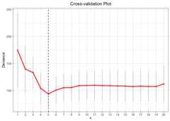
# Single Model Fit using L0 penaltyfit<-glmtlp(gau_data$X, gau_data$y,family ="gaussian",penalty ="l0")coef(fit,kappa = cv.fit$kappa.min)#> intercept V1 V2 V3 V4 V5#> -0.009687042 1.240319880 0.000000000 0.000000000 0.000000000 0.000000000#> V6 V7 V8 V9 V10 V11#> 0.883378583 0.000000000 0.000000000 0.000000000 0.725607300 0.000000000#> V12 V13 V14 V15 V16 V17#> 0.000000000 0.000000000 0.000000000 1.125958218 0.000000000 0.000000000#> V18 V19 V20#> 0.000000000 0.000000000 0.981544178predict(fit,X = gau_data$X[1:5, ],kappa = cv.fit$kappa.min)#> [1] 0.190596 2.228306 -1.425994 0.931749 -2.815322plot(fit,xvar ="kappa",label =TRUE)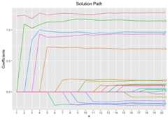
# Cross-Validation using L1 penaltycv.fit<-cv.glmtlp(gau_data$X, gau_data$y,family ="gaussian",penalty ="l1",ncores=2)coef(cv.fit)[abs(coef(cv.fit))>0]#> intercept V1 V3 V4 V5 V6#> -0.01185622 1.16222899 -0.06606911 -0.08387185 -0.06870578 0.79106593#> V8 V9 V10 V11 V14 V15#> 0.01136376 0.01038075 0.62580166 0.10858744 0.08533479 1.04737369#> V19 V20#> -0.11859786 0.86736897plot(cv.fit)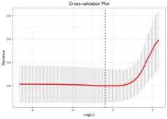
# Single Model Fit using L1 penaltyfit<-glmtlp(gau_data$X, gau_data$y,family ="gaussian",penalty ="l1")coef(fit,lambda = cv.fit$lambda.min)#> intercept V1 V2 V3 V4 V5#> -0.01185622 1.16222899 0.00000000 -0.06606911 -0.08387185 -0.06870578#> V6 V7 V8 V9 V10 V11#> 0.79106593 0.00000000 0.01136376 0.01038075 0.62580166 0.10858744#> V12 V13 V14 V15 V16 V17#> 0.00000000 0.00000000 0.08533479 1.04737369 0.00000000 0.00000000#> V18 V19 V20#> 0.00000000 -0.11859786 0.86736897predict(fit,X = gau_data$X[1:5, ],lambda = cv.fit$lambda.min)#> [1] 0.07112074 2.17093497 -1.09936871 0.46108771 -2.25111685plot(fit,xvar ="lambda",label =TRUE)
Examples for LogisticRegression Models
The following are three examples which show you how to useglmtlp to fit logistic regression models:
data("bin_data")colnames(bin_data$X)[bin_data$beta!=0]#> [1] "V1" "V6" "V10" "V15" "V20"# Cross-Validation using TLP penaltycv.fit<-cv.glmtlp(bin_data$X, bin_data$y,family ="binomial",penalty ="tlp",ncores=2)coef(cv.fit)[abs(coef(cv.fit))>0]#> intercept V6 V20#> -0.1347141 0.8256183 0.9940325plot(cv.fit)#> Warning: Removed 98 rows containing missing values or values outside the scale range#> (`geom_line()`).#> Warning: Removed 98 rows containing missing values or values outside the scale range#> (`geom_point()`).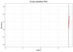
# Single Model Fit using TLP penaltyfit<-glmtlp(bin_data$X, bin_data$y,family ="binomial",penalty ="tlp")coef(fit,lambda = cv.fit$lambda.min)#> intercept V1 V2 V3 V4 V5 V6#> -0.1347141 0.0000000 0.0000000 0.0000000 0.0000000 0.0000000 0.8256183#> V7 V8 V9 V10 V11 V12 V13#> 0.0000000 0.0000000 0.0000000 0.0000000 0.0000000 0.0000000 0.0000000#> V14 V15 V16 V17 V18 V19 V20#> 0.0000000 0.0000000 0.0000000 0.0000000 0.0000000 0.0000000 0.9940325predict(fit,X = bin_data$X[1:5, ],type ="response",lambda = cv.fit$lambda.min)#> [1] 0.42562483 0.89838483 0.09767039 0.90898462 0.20822294plot(fit,xvar ="log_lambda",label =TRUE)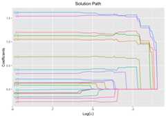
# Cross-Validation using L0 penaltycv.fit<-cv.glmtlp(bin_data$X, bin_data$y,family ="binomial",penalty ="l0",ncores=2)coef(cv.fit)[abs(coef(cv.fit))>0]#> intercept V6 V20#> -0.1347137 0.8256471 0.9940180plot(cv.fit)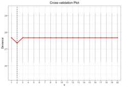
# Single Model Fit using L0 penaltyfit<-glmtlp(bin_data$X, bin_data$y,family ="binomial",penalty ="l0")coef(fit,kappa = cv.fit$kappa.min)#> intercept V1 V2 V3 V4 V5 V6#> -0.1347137 0.0000000 0.0000000 0.0000000 0.0000000 0.0000000 0.8256471#> V7 V8 V9 V10 V11 V12 V13#> 0.0000000 0.0000000 0.0000000 0.0000000 0.0000000 0.0000000 0.0000000#> V14 V15 V16 V17 V18 V19 V20#> 0.0000000 0.0000000 0.0000000 0.0000000 0.0000000 0.0000000 0.9940180predict(fit,X = bin_data$X[1:5, ],kappa = cv.fit$kappa.min)#> [1] -0.2996886 2.1793764 -2.2234461 2.3012922 -1.3357999plot(fit,xvar ="kappa",label =TRUE)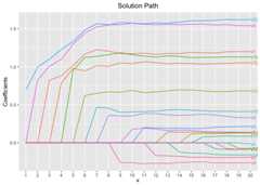
# Cross-Validation using L1 penaltycv.fit<-cv.glmtlp(bin_data$X, bin_data$y,family ="binomial",penalty ="l1",ncores=2)coef(cv.fit)[abs(coef(cv.fit))>0]#> intercept V1 V3 V4 V5 V6#> -0.04597434 0.74281436 0.04345031 0.15993696 0.05100859 0.98672196#> V8 V9 V10 V13 V15 V19#> -0.04488821 -0.06456282 0.66422939 0.33826482 0.69062166 0.23686317#> V20#> 1.01116571plot(cv.fit)
# Single Model Fit using L1 penaltyfit<-glmtlp(bin_data$X, bin_data$y,family ="binomial",penalty ="l1")coef(fit,lambda = cv.fit$lambda.min)#> intercept V1 V2 V3 V4 V5#> -0.04597434 0.74281436 0.00000000 0.04345031 0.15993696 0.05100859#> V6 V7 V8 V9 V10 V11#> 0.98672196 0.00000000 -0.04488821 -0.06456282 0.66422939 0.00000000#> V12 V13 V14 V15 V16 V17#> 0.00000000 0.33826482 0.00000000 0.69062166 0.00000000 0.00000000#> V18 V19 V20#> 0.00000000 0.23686317 1.01116571predict(fit,X = bin_data$X[1:5, ],type ="response",lambda = cv.fit$lambda.min)#> [1] 0.35132374 0.90851038 0.03822033 0.93657911 0.03253188plot(fit,xvar ="lambda",label =TRUE)
Citing information
If you find this project useful, please consider citing
@article{ author = {Chunlin Li, Yu Yang, Chong Wu, Xiaotong Shen, Wei Pan}, title = {{glmtlp: An R package for truncated Lasso penalty}}, year = {2022}}References
Li, C., Shen, X., & Pan, W. (2021). Inference for a largedirected graphical model with interventions.arXiv preprintarXiv:2110.03805.https://arxiv.org/abs/2110.03805.
Shen, X., Pan, W., & Zhu, Y. (2012). Likelihood-based selectionand sharp parameter estimation.Journal of the American StatisticalAssociation, 107(497), 223-232.https://doi.org/10.1080/01621459.2011.645783.
Shen, X., Pan, W., Zhu, Y., & Zhou, H. (2013). On constrained andregularized high-dimensional regression.Annals of the Institute ofStatistical Mathematics, 65(5), 807-832.https://doi.org/10.1007/s10463-012-0396-3.
Tibshirani, R., Bien, J., Friedman, J., Hastie, T., Simon, N.,Taylor, J., & Tibshirani, R. J. (2012). Strong rules for discardingpredictors in lasso‐type problems.Journal of the Royal StatisticalSociety: Series B (Statistical Methodology), 74(2), 245-266.https://doi.org/10.1111/j.1467-9868.2011.01004.x.
Yang, Y. & Zou, H. A coordinate majorization descent algorithmfor l1 penalized learning.Journal of Statistical Computation andSimulation 84.1 (2014): 84-95.https://doi.org/10.1080/00949655.2012.695374.
Zhu, Y., Shen, X., & Pan, W. (2020). On high-dimensionalconstrained maximum likelihood inference.Journal of the AmericanStatistical Association, 115(529), 217-230.https://doi.org/10.1080/01621459.2018.1540986.
Zhu, Y. (2017). An augmented ADMM algorithm with application to thegeneralized lasso problem.Journal of Computational and GraphicalStatistics, 26(1), 195-204.https://doi.org/10.1080/10618600.2015.1114491.
Part of the code is adapted fromglmnet,ncvreg,andbiglasso.
Warm thanks to the authors of above open-sourcedsoftwares.
[8]ページ先頭