
The objective of plsmmLasso is to facilitate the estimation of aRegularized Partial Linear Semiparametric Mixed-Effects Model (PLSMM)through a dictionary approach for modeling the nonparametric component.The model employs a set of bases functions and automatically selectsthem using a lasso penalty. Additionally, it conducts variable selectionon the fixed-effects using another lasso penalty. The implementationalso supports the inclusion of a random intercept.
You can install the development version of plsmmLasso fromGitHub with:
# install.packages("devtools")devtools::install_github("Sami-Leon/plsmmLasso")Here’s a basic example using a simulated dataset to demonstrate howto utilize the main functions of the plsmmLasso package. This exampleassumes an effect of a grouping variable and different nonlinearfunctions for each group.
library(plsmmLasso)# Simulate a datasetset.seed(123)data_sim<-simulate_group_inter(N =50,n_mvnorm =3,grouped =TRUE,timepoints =3:5,nonpara_inter =TRUE,sample_from =seq(0,52,13),cos =FALSE,A_vec =c(1,1.5))sim<- data_sim$sim# Fit the datax<-as.matrix(sim[,-1:-3])y<- sim$yseries<- sim$seriest<- sim$tbases<-create_bases(t)lambda<-0.0046gamma<-0.00001plsmm_output<-plsmm_lasso(x, y, series, t,name_group_var ="group", bases$bases,gamma = gamma,lambda = lambda,timexgroup =TRUE,criterion ="BIC")One of the most important output of theplsmm_lasso()function is the estimates of the fixed-effects.
plsmm_output$lasso_output$theta#> Intercept group x1 x2 x3 x4 x5#> 0.19729689 3.15155151 1.91905369 0.74891414 0.02274130 0.01291499 0.01049015Here, we observe that some covariates have small values, but most arenon-zero. If we desire more regularization for the fixed-effects, we canuse a larger value for lambda.
lambda<-0.1plsmm_output<-plsmm_lasso(x, y, series, t,name_group_var ="group", bases$bases,gamma = gamma,lambda = lambda,timexgroup =TRUE,criterion ="BIC")plsmm_output$lasso_output$theta#> Intercept group x1 x2 x3 x4 x5#> 3.5544003 0.4262652 0.0000000 0.0000000 0.0000000 0.0000000 0.0000000With a larger lasso penalty, more coefficients are set to zero.
The coefficients associated with the nonlinear functions are denotedby alpha.
head(plsmm_output$lasso_output$alpha)#> [1] -5.576108e-02 -4.720350e-01 -8.130512e-03 2.368476e-10 -7.129181e-06#> [6] 0.000000e+00Similar behavior would be observed for the alpha values if we were toincrease the value of gamma.
To find optimal values for gamma and lambda, we tune thesehyperparameters using BIC-type criteria with thetune_plsmm() function and a grid search.
lambdas<- gammas<-round(exp(seq(log(1),log(1*0.00001),length.out =5)),digits =5)tuned_plsmm<-tune_plsmm(x, y, series, t,name_group_var ="group", bases$bases,gamma_vec = gammas,lambda_vec = lambdas,timexgroup =TRUE,criterion ="BIC")Thetune_plsmm() function tries every possiblecombination of the values from lambdas and gammas and returns the modelwith the best BIC (other options are BICC and EBIC). This example is forillustration purposes only; in practice, a more exhaustive grid shouldbe used.
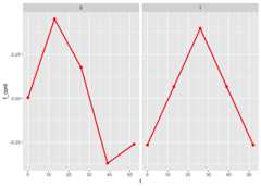
Theplot_fit() function allows for the visualization ofthe estimated mean trajectories as well as the estimate of the nonlinearfunctions. By default, only the observed time points are being used. Touse continuous time points, the argumentpredicted can beset toTRUE.
plot_fit(x, y, series, t,name_group_var ="group", tuned_plsmm)
plot_fit(x, y, series, t,name_group_var ="group", tuned_plsmm,predicted =TRUE)

To compute p-values on the fixed-effects, thedebias_plsmm() function can be used.
debias_plsmm(x, y, series, tuned_plsmm)#> Estimate Debiased Std. Error Lower 95% Upper 95% p-value#> group 3.20441442 3.31447827 0.33608394 2.65575376 3.9732028 6.079223e-23#> x1 1.95569696 2.03694234 0.21339004 1.61869786 2.4551868 1.352832e-21#> x2 0.72925412 0.68895582 0.26577859 0.16802979 1.2098818 9.535955e-03#> x3 0.02755599 0.03780433 0.04645279 -0.05324313 0.1288518 4.157466e-01#> x4 0.01691564 0.02535323 0.04110770 -0.05521786 0.1059243 5.373988e-01#> x5 0.01569818 0.02732562 0.04056090 -0.05217374 0.1068250 5.005061e-01The function reports the original coefficients, debiasedcoefficients, standard errors, confidence intervals and p-values. Thesep-values are already adjusted for the selection process of the lasso,and provide valid inference.
Finally, we can perform tests on the nonlinear functions. The firstelement of the list is an overall test of equality. If the p-value is\(< 0.05\), we reject the nullhypothesis of equality and conclude that overall the two nonlinearfunctions are different. To obtain a comparison at each time point,confidence bands are computed, and a figure displaying these confidencebands is generated. For the time points associated with confidence bandsthat include\(0\), we cannot rejectthe null hypothesis that the nonlinear functions are the same for thistime point. The data frame that is used to generate this figure can befound in the second element of the output list.
test_f_results<-test_f(x, y, series, t,name_group_var ="group", tuned_plsmm,n_boot =10,verbose =TRUE)#> | | | 0% | |======= | 10% | |============== | 20% | |===================== | 30% | |============================ | 40% | |=================================== | 50% | |========================================== | 60% | |================================================= | 70% | |======================================================== | 80% | |=============================================================== | 90% | |======================================================================| 100%#>#> Completed fitting Bootstrap samples. Now formatting results, and generating figure.
test_f_results[[1]]#> T p-value#> 1 0.4785269 0head(test_f_results[[2]])#> t f diff. Lower 95% Upper 95%#> 1 0.0 0.2365327 0.00586791 0.4414301#> 2 0.1 0.2400843 0.01051297 0.4443028#> 3 0.2 0.2436013 0.01512247 0.4471456#> 4 0.3 0.2470832 0.01969562 0.4499582#> 5 0.4 0.2505294 0.02423163 0.4527404#> 6 0.5 0.2539394 0.02872971 0.4554919Similarly to theplot_fit() function, the argumentpredicted can be changed toTRUE to displaythe joint confidence bands as a continuous function of time rather thanat the observed time points only.
test_f_results<-test_f(x, y, series, t,name_group_var ="group", tuned_plsmm,n_boot =10,predicted =TRUE)#> | | | 0% | |======= | 10% | |============== | 20% | |===================== | 30% | |============================ | 40% | |=================================== | 50% | |========================================== | 60% | |================================================= | 70% | |======================================================== | 80% | |=============================================================== | 90% | |======================================================================| 100%#>#> Completed fitting Bootstrap samples. Now formatting results, and generating figure.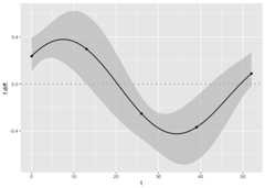
The plsmmLasso package offers flexibility; if the nonlinear functionsdo not differ between groups, thetimexgroup argument canbe set toFALSE. Below, we simulate a dataset where thenonlinear functions are the same and fit the data accordingly.
# Simulate a dataset with equal nonlinear functions per groupset.seed(123)data_sim<-simulate_group_inter(N =50,n_mvnorm =3,grouped =TRUE,timepoints =3:5,nonpara_inter =FALSE,sample_from =seq(0,52,13),cos =FALSE,A_vec =c(1,1.5))sim<- data_sim$sim# Fit the datax<-as.matrix(sim[,-1:-3])y<- sim$yseries<- sim$seriest<- sim$tbases<-create_bases(t)tuned_plsmm<-tune_plsmm(x, y, series, t,name_group_var ="group", bases$bases,gamma_vec = gammas,lambda_vec = lambdas,timexgroup =FALSE,criterion ="BIC")plot_fit(x, y, series, t,name_group_var ="group", tuned_plsmm)

As observed, the estimates of the nonlinear functions areidentical.
It is also possible not to use any grouping variable for thename_group_var argument. Here, we simulate a datasetwithout the effect of a grouping variable, resulting in no difference inthe height of the overall mean trajectories and using the same nonlinearfunctions.
# Simulate a dataset with no group effectset.seed(123)data_sim<-simulate_group_inter(N =50,n_mvnorm =3,grouped =FALSE,timepoints =3:5,nonpara_inter =FALSE,sample_from =seq(0,52,13),cos =FALSE,A_vec =c(1,1.5))sim<- data_sim$sim# Fit the datax<-as.matrix(sim[,-1:-3])y<- sim$yseries<- sim$seriest<- sim$tbases<-create_bases(t)tuned_plsmm<-tune_plsmm(x, y, series, t,name_group_var =NULL, bases$bases,gamma_vec = gammas,lambda_vec = lambdas,timexgroup =FALSE,criterion ="BIC")plot_fit(x, y, series, t,name_group_var =NULL, tuned_plsmm)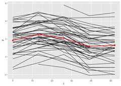
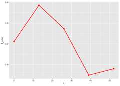
Only one figure is displayed now since there is no groupingvariable.