Movatterモバイル変換

TheARCensReg Rpackage

TheARCensReg package fits a univariate censored linearregression model with autoregressive (AR) errors. The discrete-timerepresentation of this model for the observed response at timet is given by

Y_t = x_t^⊤β + ξ_t,

ξ_t = ϕ₁ξ_t − 1 + ϕ₂ξ_t − 2 + … + ϕ_pξ_t − p + η_t,  t = 1, …, p, p + 1, …, n,

whereY_t is the response variable,β is a vector of regression parameters of dimensionl,x_t is a vector of non-stochastic regressorvariables, andξ_t is the AR error withη_t representing the innovations andϕ denoting the vector of AR coefficients. For the innovationsη_t, we consider the normal or the Student-tdistribution. The maximum likelihood estimates are obtained through theStochastic Approximation Expectation-Maximization (SAEM) algorithm(Delyon, Lavielle, and Moulines 1999), while the standard errors of theparameters are approximated by the Louis method (Louis 1982). Thispackage also predicts future observations and supports missing values onthe dependent variable. See, for instance, (Schumacher, Lachos, and Dey2017) and (Valeriano et al. 2021).

For the normal model, influence diagnostic could be performed by alocal influence approach (Cook 1986) with three possible perturbationschemes: response perturbation, scale matrix perturbation, orexplanatory variable perturbation. For more details see (Schumacher etal. 2018).

TheARCensReg package provides the followingfunctions:

• ARCensReg: fits a univariate censored linear regressionmodel with autoregressive errors under the normal distribution.
• ARtCensReg: fits a univariate censored linearregression model with autoregressive errors considering Student-tinnovations.
• InfDiag: performs influence diagnostic by a localinfluence approach with three possible perturbation schemes.
• rARCens: simulates a censored response variable withautoregressive errors of orderp.
• residuals: computes conditional and quantileresiduals.

predict,print,summary, andplot functions also work for objects given as an output offunctionsARCensReg andARtCensReg. Functionplot also has methods for outputs of functionsInfDiag andresiduals.

Next, we will describe how to install the package and use all theprevious methods in artificial examples.

Installation

The released version ofARCensReg fromCRAN can be installed with:

install.packages("ARCensReg")

And the development version fromGitHub with:

# install.packages("devtools")devtools::install_github("fernandalschumacher/ARCensReg")

Examples

Example 1. We simulated a dataset of lengthn = 100 from the autoregressive model of orderp = 2with normal innovations and left censoring.

library(ARCensReg)library(ggplot2)set.seed(12341)n=100x=cbind(1,runif(n))dat=rARCens(n=n,beta=c(1,-1),phi=c(.48,-0.4),sig2=.5,x=x,cens='left',pcens=.05,innov="norm")ggplot(dat$data,aes(x=1:n,y=y))+geom_line()+labs(x="Time")+theme_bw()+geom_line(aes(x=1:n,y=ucl),color="red",linetype="dashed")

Supposing the AR order is unknown, we fit a censored linearregression model with Gaussian AR errors of orderp = 1 andp = 2, and the information criteria are compared.

fit1=ARCensReg(dat$data$cc, dat$data$lcl, dat$data$ucl, dat$data$y, x,p=1,pc=0.15,show_se=FALSE,quiet=TRUE)fit1$critFin#>         Loglik     AIC     BIC AICcorr#> Value -113.027 234.054 244.475 234.475fit2=ARCensReg(dat$data$cc, dat$data$lcl, dat$data$ucl, dat$data$y, x,p=2,pc=0.15,quiet=TRUE)fit2$critFin#>         Loglik     AIC     BIC AICcorr#> Value -105.279 220.558 233.583 221.196

Based on the information criteria AIC and BIC, the model with ARerrors of orderp = 2 is the best fit for this data. Theparameter estimates and standard errors can be visualized throughfunctionssummary andprint.

summary(fit2)#> ---------------------------------------------------#>   Censored Linear Regression Model with AR Errors#> ---------------------------------------------------#> Call:#> ARCensReg(cc = dat$data$cc, lcl = dat$data$lcl, ucl = dat$data$ucl,#>     y = dat$data$y, x = x, p = 2, pc = 0.15, quiet = TRUE)#>#> Estimated parameters:#>       beta0   beta1 sigma2   phi1    phi2#>      1.0830 -1.0965 0.4713 0.4690 -0.3883#> s.e. 0.1465  0.2389 0.0689 0.0949  0.0941#>#> Model selection criteria:#>         Loglik     AIC     BIC AICcorr#> Value -105.279 220.558 233.583 221.196#>#> Details:#> Type of censoring: left#> Number of missing values: 0#> Convergence reached?:#> Iterations: 168 / 400#> MC sample: 10#> Cut point: 0.15#> Processing time: 44.76831 secs

Moreover, for censored data, the convergence plot of the parameterestimates can be displayed through functionplot.

plot(fit2)

Now, we perturb the observation 81 by making it equal to 6 and thenfit a censored linear regression model with Gaussian AR errors of orderp = 2.

y2= dat$data$yy2[81]=6fit3=ARCensReg(dat$data$cc, dat$data$lcl, dat$data$ucl, y2, x,p=2,show_se=FALSE,quiet=TRUE)fit3$tab#>   beta0   beta1 sigma2   phi1    phi2#>  1.1702 -1.2065 0.7237 0.3812 -0.3355

It is worth noting that the parameter estimates were affected becauseof the perturbation. Thence, we can perform influence diagnostic toidentify influential points which may cause unwanted effects onestimation and goodness of fit. In the following analysis, we onlyconsider the response perturbation scheme, where we deduced thatobservations 80 to 82 may be influential.

M0y=InfDiag(fit3,k=3.5,perturbation="y")#> Perturbation scheme: y#> Benchmark: 0.059#> Detected points: 80 81 82plot(M0y)

Example 2. A dataset of sizen = 200 issimulated from the censored regression model with Student-t innovationsand right censoring. To fit this data, we can use the functionARtCensReg, but it is worth mentioning that this functiononly works for response vectors with the firstp values whollyobserved.

set.seed(783796)n=200x=cbind(1,runif(n))dat2=rARCens(n=n,beta=c(2,1),phi=c(.48,-.2),sig2=.5,x=x,cens='right',pcens=.05,innov='t',nu=3)head(dat2$data)#>           y cc      lcl ucl#> 1 3.3242078  0 4.284143 Inf#> 2 2.9409784  0 4.284143 Inf#> 3 3.5386525  0 4.284143 Inf#> 4 3.4107191  0 4.284143 Inf#> 5 0.3564079  0 4.284143 Inf#> 6 2.6332103  0 4.284143 Inf

For models with Student-t innovations, the degrees of freedom can beprovided through argumentnufix when it is known, or thealgorithm will estimate it when it is not provided, i.e.,nufix=NULL.

# Fitting the model with nu knownfit1=ARtCensReg(dat2$data$cc, dat2$data$lcl, dat2$data$ucl, dat2$data$y, x,p=2,M=20,nufix=3,quiet=TRUE)fit1$tab#>       beta0  beta1 sigma2   phi1    phi2#>      1.9707 0.9594 0.4468 0.3778 -0.1562#> s.e. 0.1230 0.1890 0.0640 0.0572  0.0590# Fitting the model with nu unknownfit2=ARtCensReg(dat2$data$cc, dat2$data$lcl, dat2$data$ucl, dat2$data$y, x,p=2,M=20,quiet=TRUE)fit2$tab#>       beta0  beta1 sigma2   phi1    phi2     nu#>      1.9630 0.9720 0.4812 0.3798 -0.1563 3.4760#> s.e. 0.1266 0.1953 0.0991 0.0592  0.0606 1.1295

Note that the parameter estimates obtained from both models areclose, and the estimate ofν was close to the true value(ν = 3).

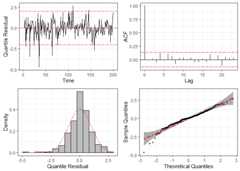
To check the statistical model’s specification, we can use graphicalmethods based on the quantile residuals, which are computed throughfunctionresiduals and plotted by functionplot.

res=residuals(fit2)plot(res)

For comparison, we fit the same dataset considering the normaldistribution (i.e., disregarding the heavy tails) and compute thecorresponding quantile residuals. The resulting plots are given below,where we can see clear signs of non-normality, such as large residualsand some points outside the confidence band in the Q-Q plots.

fit3=ARCensReg(dat2$data$cc, dat2$data$lcl, dat2$data$ucl, dat2$data$y, x,p=2,M=20,show_se=FALSE,quiet=TRUE)plot(residuals(fit3))

References