lvmisc is a package with miscellaneous R functions,including basic data computation/manipulation, easy plotting and toolsfor working with statistical models objects. You can learn more aboutthe methods for working with models invignette("working_with_models").
You can install the released version of lvmisc fromCRAN with:
install.packages("lvmisc")And the development version fromGitHub with:
# install.packages("devtools")devtools::install_github("verasls/lvmisc")Some of what you can do with lvmisc.
library(lvmisc)library(dplyr)# Compute body mass index (BMI) and categorize itstarwars%>%select(name, birth_year, mass, height)%>%mutate(BMI =bmi(mass, height/100),BMI_category =bmi_cat(BMI) )#> # A tibble: 87 × 6#> name birth_year mass height BMI BMI_category#> <chr> <dbl> <dbl> <int> <dbl> <fct>#> 1 Luke Skywalker 19 77 172 26.0 Overweight#> 2 C-3PO 112 75 167 26.9 Overweight#> 3 R2-D2 33 32 96 34.7 Obesity class I#> 4 Darth Vader 41.9 136 202 33.3 Obesity class I#> 5 Leia Organa 19 49 150 21.8 Normal weight#> 6 Owen Lars 52 120 178 37.9 Obesity class II#> 7 Beru Whitesun lars 47 75 165 27.5 Overweight#> 8 R5-D4 NA 32 97 34.0 Obesity class I#> 9 Biggs Darklighter 24 84 183 25.1 Overweight#> 10 Obi-Wan Kenobi 57 77 182 23.2 Normal weight#> # … with 77 more rows# Divide numerical variables in quantilesdivide_by_quantile(mtcars$wt,4)#> [1] 2 2 1 2 3 3 3 2 2 3 3 4 4 4 4 4 4 1 1 1 1 3 3 4 4 1 1 1 2 2 3 2#> Levels: 1 2 3 4# Center and scale variables by groupcenter_variable(iris$Petal.Width,by = iris$Species,scale =TRUE)#> [1] -0.046 -0.046 -0.046 -0.046 -0.046 0.154 0.054 -0.046 -0.046 -0.146#> [11] -0.046 -0.046 -0.146 -0.146 -0.046 0.154 0.154 0.054 0.054 0.054#> [21] -0.046 0.154 -0.046 0.254 -0.046 -0.046 0.154 -0.046 -0.046 -0.046#> [31] -0.046 0.154 -0.146 -0.046 -0.046 -0.046 -0.046 -0.146 -0.046 -0.046#> [41] 0.054 0.054 -0.046 0.354 0.154 0.054 -0.046 -0.046 -0.046 -0.046#> [51] 0.074 0.174 0.174 -0.026 0.174 -0.026 0.274 -0.326 -0.026 0.074#> [61] -0.326 0.174 -0.326 0.074 -0.026 0.074 0.174 -0.326 0.174 -0.226#> [71] 0.474 -0.026 0.174 -0.126 -0.026 0.074 0.074 0.374 0.174 -0.326#> [81] -0.226 -0.326 -0.126 0.274 0.174 0.274 0.174 -0.026 -0.026 -0.026#> [91] -0.126 0.074 -0.126 -0.326 -0.026 -0.126 -0.026 -0.026 -0.226 -0.026#> [101] 0.474 -0.126 0.074 -0.226 0.174 0.074 -0.326 -0.226 -0.226 0.474#> [111] -0.026 -0.126 0.074 -0.026 0.374 0.274 -0.226 0.174 0.274 -0.526#> [121] 0.274 -0.026 -0.026 -0.226 0.074 -0.226 -0.226 -0.226 0.074 -0.426#> [131] -0.126 -0.026 0.174 -0.526 -0.626 0.274 0.374 -0.226 -0.226 0.074#> [141] 0.374 0.274 -0.126 0.274 0.474 0.274 -0.126 -0.026 0.274 -0.226# Quick and easy plotting with {ggplot}plot_scatter(mtcars, disp, mpg,color =factor(cyl))
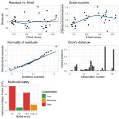
# Work with statistical model objectsm<-lm(disp~ mpg+ hp+ cyl+ mpg:cyl, mtcars)accuracy(m)#> AIC BIC R2 R2_adj MAE MAPE RMSE#> 1 344.64 353.43 0.87 0.85 34.9 15.73% 43.75plot_model(m)