Movatterモバイル変換

Introduction

@heckmanvytlacil2005eintroduced the marginal treatment effect (MTE) to provide achoice-theoretic interpretation for the widely used instrumentalvariables model of@imbensangrist1994e. The MTE canbe used to formally extrapolate from the compliers to estimate treatmenteffects for other subpopulations.

Theivmte package provides a flexible set of methodsfor conducting this extrapolation. The package uses the moment-basedframework developed by@mogstadsantostorgovitsky2018e,which accommodates both point identification and partial identification(bounds), both parametric and nonparametric models, and allows the userto maintain additional shape constraints.

Scope of this Vignette

This vignette is intended as a guide to usingivmtefor users already familiar with MTE methods. The key defintions andconcepts from that literature are used without further explanation. Wehave written a paper[@sheatorgovitsky2021wp] thatdiscusses both the MTE methodology and the usage ofivmte, which should be helpful for users unfamiliarwith MTE methods. The survey article by@mogstadtorgovitsky2018aroeprovides additional theoretical background on MTE methods, including themoment-based implementation used in this module.

Installation andRequirements

ivmte can be installed from CRAN via

install.packages("ivmte")

If you have thedevtools package, you can installthe latest version of the module directly from our GitHub repositoryvia

devtools::install_github("jkcshea/ivmte")

Two additional packages are also required forivmte:

1. splines2 for specifying models with polynomialsplines. This package is available on CRAN.
2. A package for solving linear programs. There are three options here:
   1. Gurobi and the Gurobi R packagegurobi, which canbe obtained fromGurobiOptimization. This option requires a Gurobi software license, whichGurobi Optimization offers at no cost to academic researchers.
   2. CPLEX and the packagecplexAPI, which is availableon CRAN. CPLEX can be obtained fromIBM. Thisoption requires a CPLEX software license, which IBM offers at no cost toacademic researchers.
   3. MOSEK and the packageRmosek, which can be obtainedfromMOSEK ApS. This optionrequires a MOSEK software license, which MOSEK ApS offers at no cost toacademic researchers.
   4. ThelpSolveAPI package, which is free andopen-source, and available from CRAN. Note thatlpSolveAPI is a wrapper forlp_solve, which is nolonger actively developed.

ivmte tries to automatically choose a solver fromthose available, with preference being given to Gurobi, CPLEX, andMOSEK. We have provided the option to uselpSolveAPIbecause it appears to be the only interface for solving linear programsthat can be installed solely throughinstall.packages.However, westrongly recommend using Gurobi, CPLEX, or MOSEK,since these are actively developed, much more stable, and typically anorder of magnitude faster thanlpSolveAPI. A very clearinstallation guide for Gurobi can be foundhere

Usage Demonstration

Data and Background

We will use a subsample of 209133 women from the data used in@angristevans1998taer. The datais included withivmte and has the followingstructure.

library(ivmte)knitr::kable(head(AE,n =10))

We will use these variables as follows:

• worked is a binary outcome variable that indicateswhether the woman was working.
• hours is a multivalued outcome variable that measuresthe number of hours the woman worked per week.
• morekids is a binary treatment variable that indicateswhether a woman had more than two children or exactly two children.
  • Note that@angristevans1998taer removedwomen with fewer than two children when constructing their sample.
  • Also note that the treatment variable must be binary.
• samesex is an indicator for whether the woman’s firsttwo children had the same sex (male-male or female-female). This is usedas an instrument formorekids.
• yob is the woman’s year of birth (i.e. her age), whichwill be used as a conditioning variable.

A goal of@angristevans1998taer was toestimate the causal effect ofmorekids on eitherworked orhours. A linear regression ofworked onmorekids yields:

lm(data = AE, worked~ morekids)#>#> Call:#> lm(formula = worked ~ morekids, data = AE)#>#> Coefficients:#> (Intercept)     morekids#>      0.5822      -0.1423

The regression shows that women with three or more children are about14–15% less likely to be working than women with exactly two children.Is this because children have a negative impact on a woman’s laborsupply? Or is it because women with a weaker attachment to the labormarket choose to have more children?

@angristevans1998taer addressthis question by usingsamesex as an instrument formorekids. We expect thatsamesex is randomlyassigned, so that among women with two or more children, those with weaklabor market attachment are just as likely as those with strong labormarket attachment to have to have two boys or two girls for their firsttwo children. A regression shows that women whose first two children hadthe same sex are also more likely to go on to have a third child:

lm(data = AE, morekids~ samesex)#>#> Call:#> lm(formula = morekids ~ samesex, data = AE)#>#> Coefficients:#> (Intercept)      samesex#>     0.30214      0.05887

Thus,samesex constitutes a potential instrumentalvariable formorekids. We can run a simple instrumentalvariable regression using theivreg command from theAER package.

library("AER")ivreg(data = AE, worked~ morekids| samesex )#>#> Call:#> ivreg(formula = worked ~ morekids | samesex, data = AE)#>#> Coefficients:#> (Intercept)     morekids#>     0.56315     -0.08484

The coefficient onmorekids is smaller in magnitude thanit was in the linear regression ofworked onmorekids. This suggests that the linear regressionoverstates the negative impact that children have on a woman’s laborsupply. The likely explanation is that women who have more children wereless likely to work anyway.

An important caveat to this reasoning, first discussed by@imbensangrist1994e, is that itapplies only to the group ofcompliers who would have had athird child if and only if their first two children were same sex. (Thisinterpretation requires the so-calledmonotonicity condition.)The first stage regression ofmorekids onsamesex shows that this group comprises less than 6% of theentire population. Thus, the complier subpopulation is a small andpotentially unrepresentative group of individuals.

Is the relationship between fertility and labor supply for thecompliers the same as for other groups? The answer is important if wewant to use an instrumental variable estimator to inform policyquestions. The purpose ofivmte is to provide a formalframework for answering this type of extrapolation question.

For demonstrating some of the features ofivmte, itwill also be useful to use a simulated dataset. The following code,which is contained in./extdata/ivmteSimData.R, generatessome simulated data from a simple DGP. The simulated data is alsoincluded with the package as./data/ivmteSimData.rda.

set.seed(1)n<-5000u<-runif(n)z<-rbinom(n,3, .5)x<-as.numeric(cut(rnorm(n),10))# normal discretized into 10 binsd<-as.numeric(u< z*.25+ .01*x)v0<-rnorm(n)+ .2*um0<-0y0<-as.numeric(m0+ v0+ .1*x>0)v1<-rnorm(n)- .2*um1<- .5y1<-as.numeric(m1+ v1- .3*x>0)y<- d*y1+ (1-d)*y0ivmteSimData<-data.frame(y,d,z,x)knitr::kable(head(ivmteSimData,n =10))

Syntax and Output Overview

The main command of theivmte package is also calledivmte. It has the following basic syntax:

library("ivmte")results<-ivmte(data = AE,target ="att",m0 =~ u+ yob,m1 =~ u+ yob,ivlike = worked~ morekids+ samesex+ morekids*samesex,propensity = morekids~ samesex+ yob,noisy =TRUE)

Here’s what these required parameters refer to:

• data = AE is the usual reference to the data to beused.
• target = "att" specifies the target parameter to be theaverage treatment on the treated (ATT).
• m0 andm1 are formulas specifying the MTRfunctions for the untreated and treated arms, respectively. The symbolu in the formula refers to the unobservable latent variablein the selection equation.
• ivlike indicates the regressions to be run to createmoments to which the model is fit.
• propensity specifies a model for the propensityscore.

This is what happens when the code above is run:

results<-ivmte(data = AE,target ="att",m0 =~ u+ yob,m1 =~ u+ yob,ivlike = worked~ morekids+ samesex+ morekids*samesex,propensity = morekids~ samesex+ yob,noisy =TRUE)#>#> Solver: Gurobi ('gurobi')#>#> Obtaining propensity scores...#>#> Generating target moments...#>     Integrating terms for control group...#>     Integrating terms for treated group...#>#> Generating IV-like moments...#>     Moment 1...#>     Moment 2...#>     Moment 3...#>     Moment 4...#>     Independent moments: 4#>#> Performing audit procedure...#>     Generating initial constraint grid...#>#>     Audit count: 1#>     Minimum criterion: 0#>     Obtaining bounds...#>     Violations: 0#>     Audit finished.#>#> Bounds on the target parameter: [-0.1028836, -0.07818869]

Whennoisy = TRUE, theivmte functionindicates its progress in performing a sequence of intermediateoperations. It then runs through an audit procedure to enforce shapeconstraints. The audit procedure is described in more detailahead. After the audit procedure terminates,ivmte returns bounds on the target parameter, which in thiscase is the average treatment on the treated(target = "att"). These bounds are the primary output ofinterest.

The detailed output can be suppressed by passingnoisy = FALSE as an additional parameter. By default,detailed output is suppressed. Should the user wish to review theoutput, it is returned under the entry$messages,regardless of the value of thenoisy parameter.

results<-ivmte(data = AE,target ="att",m0 =~ u+ yob,m1 =~ u+ yob,ivlike = worked~ morekids+ samesex+ morekids*samesex,propensity = morekids~ samesex+ yob,noisy =FALSE)results#>#> Bounds on the target parameter: [-0.1028836, -0.07818869]#> Audit terminated successfully after 1 roundcat(results$messages,sep ="\n")#>#> Solver: Gurobi ('gurobi')#>#> Obtaining propensity scores...#>#> Generating target moments...#>     Integrating terms for control group...#>     Integrating terms for treated group...#>#> Generating IV-like moments...#>     Moment 1...#>     Moment 2...#>     Moment 3...#>     Moment 4...#>     Independent moments: 4#>#> Performing audit procedure...#>     Generating initial constraint grid...#>#>     Audit count: 1#>     Minimum criterion: 0#>     Obtaining bounds...#>     Violations: 0#>     Audit finished.#>#> Bounds on the target parameter: [-0.1028836, -0.07818869]

Specifying the MTR Functions

Basics

The requiredm0 andm1 arguments use thestandard R formula syntax familiar from functions likelmorglm. However, the formulas involve an unobservablevariable,u, which corresponds to the latent propensity totake treatment in the selection equation. This variable can be includedin formulas in the same way as other observable variables in the data.For example,

args<-list(data = AE,ivlike =  worked~ morekids+ samesex+ morekids*samesex,target ="att",m0 =~ u+I(u^2)+ yob+ u*yob,m1 =~ u+I(u^2)+I(u^3)+ yob+ u*yob,propensity = morekids~ samesex+ yob)r<-do.call(ivmte, args)r#>#> Bounds on the target parameter: [-0.2950822, 0.1254494]#> Audit terminated successfully after 3 rounds

A restriction that we make for computational purposes is thatu can only appear in polynomial terms (perhaps interactedwith other variables). Thus, the following raises an error

args[["m0"]]<-~log(u)+ yobr<-do.call(ivmte, args)#> Error: The following terms are not declared properly.#>   m0: log(u)#> The unobserved variable 'u' must be declared as a monomial, e.g. u, I(u^3). The monomial can be interacted with other variables, e.g. x:u, x:I(u^3). Expressions where the unobservable term is not a monomial are either not permissible or will not be parsed correctly, e.g. exp(u), I((x * u)^2). Try to rewrite the expression so that 'u' is only included in monomials.

Names other thanu can be used for the selectionequation unobservable, but one must remember to pass the optionuname to indicate the new name.

args[["m0"]]<-~ v+I(v^2)+ yob+ v*yobargs[["m1"]]<-~ v+I(v^2)+I(v^3)+ yob+ v*yobargs[["uname"]]<-"v"r<-do.call(ivmte, args)r#>#> Bounds on the target parameter: [-0.2950822, 0.1254494]#> Audit terminated successfully after 3 rounds

There are some limitations regarding the use of factor variables. Forexample, the following formula form1 will trigger anerror.

args[["uname"]]<-~"u"args[["m0"]]<-~ u+ yobargs[["m1"]]<-~ u+factor(yob)55+factor(yob)60

However, one can work around this in a natural way.

args[["m1"]]<-~ u+ (yob==55)+ (yob==60)r<-do.call(ivmte, args)r#>#> Bounds on the target parameter: [-0.1028836, -0.07818869]#> Audit terminated successfully after 1 round

Polynomial Splines

In addition to global polynomials inu,ivmte also allows for polynomial splines inuusing the keyworduSplines. For example,

args<-list(data = AE,ivlike =  worked~ morekids+ samesex+ morekids*samesex,target ="att",m0 =~ u+uSplines(degree =1,knots =c(.2, .4, .6, .8))+ yob,m1 =~uSplines(degree =2,knots =c(.1, .3, .5, .7))*yob,propensity = morekids~ samesex+ yob)r<-do.call(ivmte, args)r#>#> Bounds on the target parameter: [-0.4545814, 0.3117817]#> Audit terminated successfully after 2 rounds

Thedegree refers to the polynomial degree, so thatdegree = 1 is a linear spline, anddegree = 2is a quadratic spline. Constant splines, which have an important role insome of the theory developed by@mogstadsantostorgovitsky2018e,can be implemented withdegree = 0. The vectorknots indicates the piecewise regions for the spline. Notethat0 and1 are always automatically includedasknots, so that only the interior knots need to bespecified.

Shape Restrictions

One can also require the MTR functions to satisfy the followingnonparametric shape restrictions.

• Boundedness of the MTR functions, via the parametersm0.lb,m0.ub,m1.lb, andm1.ub, which all take scalar values. In order to producenon-trivial bounds in cases of partial identification,m0.lb andm1.lb are by default set to thesmallest value of the response variable (which is inferred fromivlike) that is observed in the data, whilem0.ub andm1.ub are set to the largestvalue.
• Boundedness of the MTE function, that is,m1 - m0, bysettingmte.lb andmte.ub. By default, theseare set to the values logically implied by the values form0.lb,m0.ub,m1.lb, andm1.ub.
• Monotonicity of the MTR functions inu for each valueof the other observed variables, via the parametersm0.dec,m0.inc,m1.dec,m1.inc, which alltake boolean values.
• Monotonicity of the MTE function inu, via theparametersmte.dec andmte.inc.

Here is an example with monotonicity restrictions:

args<-list(data = AE,ivlike =  worked~ morekids+ samesex+ morekids*samesex,target ="att",m0 =~ u+uSplines(degree =1,knots =c(.2, .4, .6, .8))+ yob,m1 =~uSplines(degree =2,knots =c(.1, .3, .5, .7))*yob,m1.inc =TRUE,m0.inc =TRUE,mte.dec =TRUE,propensity = morekids~ samesex+ yob)r<-do.call(ivmte, args)r#>#> Bounds on the target parameter: [-0.09769381, 0.09247149]#> Audit terminated successfully after 1 round

The Audit Procedure

The shape restrictions in the previous section are enforced by addingconstraints to a linear program. It is difficult in general to ensurethat a function satisfies restrictions such as boundedness ormonotonicity, even if that function is known to be a polynomial. Thisdifficulty is addressed inivmte through an auditingprocedure.

The auditing procedure is based on two grids: A relatively smallconstraint grid, and a relatively largeaudit grid.The MTR functions (and implied MTE function) are made to satisfy thespecified shape restrictions on the constraint grid by addingconstraints to the linear programs. While this ensures that the MTRfunctions satisfy the shape restrictions on the constraint grid, it doesnot ensure that they satisfy the restrictions “everywhere.” Thus, aftersolving the programs, we evaluate the solution MTR functions on thelarge audit grid, which is relatively inexpensive computationally. Ifthere are points in the audit grid at which the solution MTRs violatethe desired restrictions, then we add some of these points to theconstraint grid and repeat the procedure. The procedure ends (the auditis passed), when the solution MTRs satisfy the constraints over theentire audit grid.

There are certain parameters that can be used to tune the auditprocedure: The number of initial points in the constraint grid(initgrid.nu andinitgrid.nx), the number ofpoints in the audit grid (audit.nu andaudit.nx), the maximum number of points that are added fromthe audit grid to the constraint grid (audit.add) for eachconstraint, and the maximum number of times the audit procedure isrepeated before giving up (audit.max). We have tried tochoose defaults for these parameters that should be suitable for mostapplications. However, ifivmte takes a very long time torun, one might want to try adjusting these parameters. Also, ifaudit.max is hit, which should be unlikely given thedefault settings, one should either adjust the settings or examine theaudit.grid$violations field of the returned results to seethe extent to which the shape restrictions are not satisfied.

Specifying the TargetParameter

The target parameter is the object the researcher wants to know.ivmte has built-in support for conventional targetparameters and a class of generalized LATEs. It also has a system thatallows users to construct their own target parameters by defining theassociated weights.

Conventional TargetParameters

The target parameter can be set to the average treatment effect(ATE), average treatment on the treated (ATT), or the average treatmenton the untreated by settingtarget toate,att, oratu, respectively. For example:

args<-list(data = AE,ivlike =  worked~ morekids+ samesex+ morekids*samesex,target ="att",m0 =~ u+I(u^2)+ yob+ u*yob,m1 =~ u+I(u^2)+I(u^3)+ yob+ u*yob,propensity = morekids~ samesex+ yob)r<-do.call(ivmte, args)r#>#> Bounds on the target parameter: [-0.2950822, 0.1254494]#> Audit terminated successfully after 3 roundsargs[["target"]]<-"ate"r<-do.call(ivmte, args)r#>#> Bounds on the target parameter: [-0.375778, 0.1957841]#> Audit terminated successfully after 1 round

LATEs and Generalized LATEs

LATEs can be set as target parameters by passingtarget = late and including named lists calledlate.from andlate.to. The named lists shouldcontain variable name and value pairs, where the variable names mustalso appear in the propensity score formula. Typically, one would chooseinstruments for these variables, althoughivmte will letyou include control variables as well. We demonstrate this using thesimulated data.

args<-list(data = ivmteSimData,ivlike =  y~ d+ z+ d*z,target ="late",late.from =c(z =1),late.to =c(z =3),m0 =~ u+I(u^2)+I(u^3)+ x,m1 =~ u+I(u^2)+I(u^3)+ x,propensity = d~ z+ x)r<-do.call(ivmte, args)r#>#> Bounds on the target parameter: [-0.6931532, -0.4397993]#> Audit terminated successfully after 2 rounds

We can condition on covariates in the definition of the LATE byadding the named listlate.X as follows.

args[["late.X"]]=c(x =2)r<-do.call(ivmte, args)r#>#> Bounds on the target parameter: [-0.8419396, -0.2913049]#> Audit terminated successfully after 2 roundsargs[["late.X"]]=c(x =8)r<-do.call(ivmte, args)r#>#> Bounds on the target parameter: [-0.7721625, -0.3209851]#> Audit terminated successfully after 2 rounds

ivmte also provides support for generalized LATEs,i.e. LATEs where the intervals ofu that are beingconsidered may or may not correspond to points in the support of thepropensity score. These objects are useful for a number of extrapolationpurposes, see e.g.@mogstadsantostorgovitsky2018e.They are set withtarget = "genlate" and the additionalscalarsgenlate.lb andgenlate.ub. Forexample,

args<-list(data = ivmteSimData,ivlike =  y~ d+ z+ d*z,target ="genlate",genlate.lb = .2,genlate.ub = .4,m0 =~ u+I(u^2)+I(u^3)+ x,m1 =~ u+I(u^2)+I(u^3)+ x,propensity = d~ z+ x)r<-do.call(ivmte, args)args[["genlate.ub"]]<- .41r<-do.call(ivmte, args)args[["genlate.ub"]]<- .42r<-do.call(ivmte, args)r#>#> Bounds on the target parameter: [-0.7504255, -0.3182317]#> Audit terminated successfully after 2 rounds

Generalized LATEs can also be made conditional-on-covariates bypassinglate.X:

args[["late.X"]]<-c(x =2)r<-do.call(ivmte, args)r#>#> Bounds on the target parameter: [-0.867551, -0.2750135]#> Audit terminated successfully after 2 rounds

Custom Target Parameters

Since there are potentially a large and diverse array of targetparameters that a researcher might be interested in across variousapplications, theivmte package also allows thespecification of custom target parameters. This is done by specifyingthe two weighting functions for the target parameters.

To facilitate computation, these functions must be expressible asconstant splines inu. For the untreated weights, the knotsof the spline are specified withtarget.knots0 and theweights to place in between each knot is given bytarget.weight0. Since the weighting functions might dependon both the instrument and other covariates, bothtarget.knots0 andtarget.weight0 should belists consisting of functions or scalars. (A scalar is interpreted as aconstant function.) If the lists include any functions, then thearguments of the functions must be the names of the variables that theknots or weights depend on. These variables do not have to be a part ofthe model, but must be included in the data provided toivmte. Specifying the treated weights works the same waybut withtarget.knots1 andtarget.weight1. Ifthetarget option is passed along with the custom weights,an error is returned.

Here is an example of using custom weights to replicate theconditional LATE from above.

pmodel<- r$propensity$model# returned from the previous run of ivmtexeval=2# x = xeval is the group that is conditioned onpx<-mean(ivmteSimData$x== xeval)# probability that x = xevalz.from=1z.to=3weight1<-function(x) {if (x!= xeval) {return(0)    }else {        xz.from<-data.frame(x = xeval,z = z.from)        xz.to<-data.frame(x = xeval,z = z.to)        p.from<-predict(pmodel,newdata = xz.from,type ="response")        p.to<-predict(pmodel,newdata = xz.to,type ="response")return(1/ ((p.to- p.from)* px))    }}weight0<-function(x) {return(-weight1(x))}## Define knots (same for treated and control)knot1<-function(x) {    xz.from<-data.frame(x = x,z = z.from)    p.from<-predict(pmodel,newdata = xz.from,type ="response")return(p.from)}knot2<-function(x) {    xz.to<-data.frame(x = x,z = z.to)    p.to<-predict.glm(pmodel,newdata = xz.to,type ="response")return(p.to)}args<-list(data = ivmteSimData,ivlike =  y~ d+ z+ d*z,target.knots0 =c(knot1, knot2),target.knots1 =c(knot1, knot2),target.weight0 =c(0, weight0,0),target.weight1 =c(0, weight1,0),m0 =~ u+I(u^2)+I(u^3)+ x,m1 =~ u+I(u^2)+I(u^3)+ x,propensity = d~ z+ x)r<-do.call(ivmte, args)r#>#> Bounds on the target parameter: [-0.8419396, -0.2913049]#> Audit terminated successfully after 2 rounds

The knot specification here is the same for both the treated anduntreated weights. It specifies two knots that depend on whetherx == 2, so that there are four knots total when accountingfor 0 and 1, which are always included automatically. These four knotsdivide the interval between 0 and 1 into three regions. The first regionis from 0 to the value of the propensity score when evaluated atx andz.from. The second region is betweenthis point and the propensity score evaluated atx andz.to. The third and final region is from this point up to1.

Since the knot specification creates three regions, three weightfunctions must be passed. Here, the weights in the first and thirdregions are set to 0 regardless of the value ofx by justpassing a scalar0. The weights in the second region areonly non-zero whenx == 2, in which case they are equal tothe inverse of the distance between the second and third knot points.Thus, the weighting scheme applies equal weight to compliers withx == 2, and zero weight to all others. As expected, theresulting bounds match those that we computed above usingtarget == late.

Specifying the IV–LikeEstimands

The IV–like estimands refer to the moments in the data that are usedto fit the model. Inivmte these are restricted to beonly moments that can be expressed as the coefficient in either a linearregression (LR) or two stage least squares (TSLS) regression of theoutcome variable on the other variables in the dataset.

There are three aspects that can be changed, which we discuss inorder subsequently. First, one can specify one or multiple LR and TSLSformulas from which moments are used. By default, all moments from eachformula are used. Second, one can specify that only certain moments froma formula are used. Third, one can specify a subset of the data on whichthe formula is run, which provides an easy way to nonparametricallycondition on observables.

List of Linear ModelFormulas

The requiredivlike option expects a list of R formulas.All of our examples up to now have had a single LR. However, one caninclude multiple LRs, as well as TSLS regressions using the| syntax familiar from theAER package.Each formula must have the same variable on the left-hand side, which ishow the outcome variable gets inferred. For example,

args<-list(data = ivmteSimData,ivlike =c(y~ (z==1)+ (z==2)+ (z==3)+ x,                         y~ d+ x,                         y~ d| z),target ="ate",m0 =~uSplines(degree =1,knots =c(.25, .5, .75))+ x,m1 =~uSplines(degree =1,knots =c(.25, .5, .75))+ x,propensity = d~ z+ x)r<-do.call(ivmte, args)#> Warning: The following IV-like specifications do not include the treatment#> variable: 1. This may result in fewer independent moment conditions than#> expected.r#>#> Bounds on the target parameter: [-0.6427017, -0.3727193]#> Audit terminated successfully after 1 round

There are 10 moments being fit in this specification. Five of thesemoments correspond to the constant term, the coefficients on the threedummies(z == 1),(z == 2) and(z == 3), and the coefficient onx from thefirst linear regression. There are three more coefficients from thesecond regression ofy ond,x,and a constant. Finally, there are two moments from the TSLS (simple IVin this case) regression ofy ond and aconstant, usingz and a constant as instruments.

Using Only Subcomponents

The default behavior ofivmte is to use all of themoments from each formula included inivlike. There arereasons one might not want to do this, such as if certain moments areestimated poorly (i.e. with substantial statistical error). For moreinformation, see the discussions in@mogstadsantostorgovitsky2018eand@mogstadtorgovitsky2018aroe.

One can tellivmte to only include certain moments andnot others by passing thecomponents option. This optionexpects a list of the same length as the list passed toivlike. Each component of the list is itself a list thatcontains the variable names for the coefficients to be included fromthat formula. The list should be declared using thelfunction, which is a generalization of thelist function.Thel function allows the user to list variables andexpressions without having to enclose them by quotation marks. Forexample, the following includes the coefficients on the intercept andx from the first formula, the coefficient ondfrom the second formula, and all coefficients in the third formula.

args[["components"]]<-l(c(intercept, x),c(d), )r<-do.call(ivmte, args)r#>#> Bounds on the target parameter: [-0.6865291, -0.2573525]#> Audit terminated successfully after 1 round

Note thatintercept is a reserved word that is used tospecify the coefficient on the constant term. If the functionlist is used to pass thecomponents option, anerror will follow.

args[["components"]]<-list(c(intercept, x),c(d), )#> Error in eval(expr, envir, enclos): object 'intercept' not foundargs[["components"]]<-list(c("intercept","x"),c("d"),"")r<-do.call(ivmte, args)#> Error in terms.formula(fi, ...): invalid model formula in ExtractVars

Subsetting

The formulas can be run conditional on certain subgroups by addingthesubset option. This option expects a list of logicalstatements with the same length asivlike declared usingthel function. One can use the entire data by leaving thestatement blank, or inserting a tautology such as1 == 1.For example, the following would run the first regression only onobservations withx less than or equal to 9, the secondregression on the entire sample, and the third (TSLS) formula only onthose observations that havez equal to 1 or 3.

args<-list(data = ivmteSimData,ivlike =c(y~ z+ x,                         y~ d+ x,                         y~ d| z),subset =l(x<=9,1==1, z%in%c(1,3)),target ="ate",m0 =~uSplines(degree =3,knots =c(.25, .5, .75))+ x,m1 =~uSplines(degree =3,knots =c(.25, .5, .75))+ x,propensity = d~ z+ x)r<-do.call(ivmte, args)#> Warning: The following IV-like specifications do not include the treatment#> variable: 1. This may result in fewer independent moment conditions than#> expected.r#>#> Bounds on the target parameter: [-0.6697228, -0.3331582]#> Audit terminated successfully after 2 rounds

Specifying the PropensityScore

The procedure implemented byivmte requires firstestimating the propensity score, that is, the probability that thebinary treatment variable is 1, conditional on the instrument and othercovariates. This must be specified with thepropensityoption, which expects a formula. The treatment variable is inferred tobe the variable on the left-hand side of thepropensity.The default is to estimate the formula as a logit model via theglm command, but this can be changed to"linear" or"probit" with thelink option.

results<-ivmte(data = AE,target ="att",m0 =~ u+ yob,m1 =~ u+ yob,ivlike = worked~ morekids+ samesex+ morekids*samesex,propensity = morekids~ samesex+ yob,link ="probit")results#>#> Bounds on the target parameter: [-0.100781, -0.0825274]#> Audit terminated successfully after 1 round

Point Identified Models

By default,ivmte will determine if the model is pointidentified. This typically occurs whenivlike,components andsubset are such that they havemore (non-redundant) components than there are free parameters inm0 andm1. If the model is point identified,then the bounds will typically shrink to a point. Theivmtefunction will then estimate the target parameter using quadratic lossand the optimal two-step GMM weighting matrix for moments. If the modelis known to be point identified beforehand, one can include the optionpoint = TRUE to ensure the target parameter is estimatedthis way. One can additionally passpoint.eyeweight = TRUEto estimate the target parameter using identity weighting.

args<-list(data = ivmteSimData,ivlike =  y~ d+factor(z),target ="ate",m0 =~ u,m1 =~ u,propensity = d~factor(z),point =TRUE)r<-do.call(ivmte, args)r#>#> Point estimate of the target parameter: -0.5389508

Ifivmte determines that the model is not pointidentified or the user passespoint = FALSE, then thebounds on the target parameter will be estimated. However, the user maystill passpoint = FALSE even though there are more(non-redundant) moments than free parameters inm0 andm1. The bounds will collapse to a point, but may differfrom the case wherepoint = TRUE. The reason is thativmte uses absolute deviation loss instead of quadraticloss whenpoint = FALSE. To demonstrate this, the examplebelow sets the tuning parametercriterion.tol = 0 so thatthe bounds indeed collapse to a point (see@mogstadsantostorgovitsky2018efor more detail).

args$point<-FALSEargs$criterion.tol<-0r<-do.call(ivmte, args)r#>#> Bounds on the target parameter: [-0.5349027, -0.5349027]#> Audit terminated successfully after 1 round

One should usepoint = TRUE if the model is pointidentified, since it computes confidence intervals and specificationtests (discussed ahead) in a well-understood way.

Confidence Intervals

Theivmte command does provide functionality forconstructing confidence regions, although this is turned off by default,since it can be computationally expensive. To turn it on, setbootstraps to be a positive integer. The confidenceintervals are stored under$bounds.ci.

r<-ivmte(data = AE,target ="att",m0 =~ u+ yob,m1 =~ u+ yob,ivlike = worked~ morekids+ samesex+ morekids*samesex,propensity = morekids~ samesex+ yob,bootstraps =50)summary(r)#>#> Bounds on the target parameter: [-0.1028836, -0.07818869]#> Audit terminated successfully after 1 round#> MTR coefficients: 6#> Independent/total moments: 4/4#> Minimum criterion: 0#> Solver: Gurobi ('gurobi')#>#> Bootstrapped confidence intervals (backward):#>     90%: [-0.1767266, 0.01163401]#>     95%: [-0.1877661, 0.0125208]#>     99%: [-0.1879194, 0.05562988]#> p-value: 0.16#> Number of bootstraps: 50

Other options relevent to confidence region construction arebootstraps.m, which indicates the number of observations todraw from the sample on each bootstrap replication, andbootstraps.replace to indicate whether these observationsshould be drawn with or without replacement. The default is to setbootstraps.m to the sample size of the observed data withbootstraps.replace = TRUE. This corresponds to the usualnonparametric bootstrap. Choosingbootstraps.m to besmaller than the sample size and settingbootstraps.replaceto beTRUE orFALSE corresponds to the “m outof n” bootstrap or subsampling, respectively. Regardless of thesesettings, two types of confidence regions are constructed following theterminology of@andrewshan2009ej; see@sheatorgovitsky2021wp formore detail, references, and important theoretical caveats to theprocedures. While thesummary output displays only thebackward confidence region, both forward and backward confidence regionsare stored under$bounds.ci.

r$bounds.ci#> $backward#>      lb.backward ub.backward#> 0.9   -0.1767266  0.01163401#> 0.95  -0.1877661  0.01252080#> 0.99  -0.1879194  0.05562988#>#> $forward#>      lb.forward   ub.forward#> 0.9  -0.2013875 -0.010580678#> 0.95 -0.2021541 -0.007122401#> 0.99 -0.2473285 -0.002190831

The bootstrapped bounds are returned and stored inr$bounds.bootstraps, and can be used to plot thedistribution of bound estimates.

head(r$bounds.bootstrap)#>          lower       upper#> 1 -0.176726565 -0.13140944#> 2 -0.079414585 -0.04838939#> 3 -0.004379649  0.01163401#> 4 -0.126917750 -0.09350509#> 5 -0.110911453 -0.09289715#> 6 -0.101183496 -0.08202556

The dashed lines in the figure below indicate the bounds obtainedfrom the original sample.

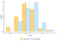
Confidence regions can also be constructed whenpoint == TRUE in a similar way. The bootstrapped pointestimates are returned and stored inr$point.estimate.bootstraps.

args<-list(data = AE,target ="att",m0 =~ u,m1 =~ u,ivlike = worked~ morekids+ samesex+ morekids*samesex,propensity = morekids~ samesex,point =TRUE,bootstraps =50)r<-do.call(ivmte, args)summary(r)#>#> Point estimate of the target parameter: -0.09160436#> MTR coefficients: 4#> Independent/total moments: 4/4#>#> Bootstrapped confidence intervals (nonparametric):#>     90%: [-0.1521216, -0.02213206]#>     95%: [-0.1595378, -0.01554401]#>     99%: [-0.2023271, -0.002062735]#> p-value: 0.02#> Number of bootstraps: 50

The p-value reported in both cases is for the null hypothesis thatthe target parameter is equal to 0, which we infer here by finding thelargest confidence region that does not contain 0. By default,ivmte returns 99%, 95%, and 90% confidence intervals. Thiscan be changed with thelevels option.

Specification Tests

The moment-based framework implemented byivmte isamenable to specification tests. These tests are based on whether theminimum value of the criterion function is statistically different from0. In the point identified case, this is the well known GMMoveridentification test[@hansen1982e]. Here, we implement itvia bootstrapping as discussed by@hallhorowitz1996e, because themoments depend on the estimated propensity score which is estimated in afirst stage. In the partially identified case, we implement themisspecification test discussed by@bugnicanayshi2015joe. Thespecification tests are automatically conducted whenbootstraps is positive and the minimum criterion value inthe sample problem is larger than 0. However, it can be turned off bysettingspecification.test = FALSE.

args<-list(data = ivmteSimData,ivlike =  y~ d+factor(z),target ="ate",m0 =~ u,m1 =~ u,m0.dec =TRUE,m1.dec =TRUE,propensity = d~factor(z),bootstraps =50)r<-do.call(ivmte, args)#> Warning: MTR is point identified via GMM. Shape constraints are ignored.summary(r)#>#> Point estimate of the target parameter: -0.5389508#> MTR coefficients: 4#> Independent/total moments: 5/5#>#> Bootstrapped confidence intervals (nonparametric):#>     90%: [-0.6085175, -0.4937168]#>     95%: [-0.6122408, -0.4929158]#>     99%: [-0.6282604, -0.4765259]#> p-value: 0#> Bootstrapped J-test p-value: 0.32#> Number of bootstraps: 50args[["ivlike"]]<- y~ d+factor(z)+ d*factor(z)# many more momentsargs[["point"]]<-TRUEr<-do.call(ivmte, args)#> Warning: If argument 'point' is set to TRUE, then shape restrictions on m0 and#> m1 are ignored, and the audit procedure is not implemented.summary(r)#>#> Point estimate of the target parameter: -0.5559325#> MTR coefficients: 4#> Independent/total moments: 8/8#>#> Bootstrapped confidence intervals (nonparametric):#>     90%: [-0.6009581, -0.5048528]#>     95%: [-0.605144, -0.5039834]#>     99%: [-0.6100535, -0.501858]#> p-value: 0#> Bootstrapped J-test p-value: 0.52#> Number of bootstraps: 50

Plotting MTRs and MTEs

After the estimation procedure, the MTR and MTE functions can beplotted for for further analysis. Below is a demonstration of how togenerate such plots when the MTR functions contain splines.

args<-list(data = AE,ivlike =  worked~ morekids+ samesex+ morekids*samesex,target ="att",m0 =~0+uSplines(degree =2,knots =c(1/3,2/3)),m1 =~0+uSplines(degree =2,knots =c(1/3,2/3)),m1.inc =TRUE,m0.inc =TRUE,mte.dec =TRUE,propensity = morekids~ samesex)r<-do.call(ivmte, args)r#>#> Bounds on the target parameter: [-0.08484221, 0.08736006]#> Audit terminated successfully after 2 rounds

The specification of each uniquely defined spline is stored in thelistr$splines.dict. For example, ifm0contained only the termsuSplines(degree = 0, knots = 0.5)andx:uSplines(degree = 0, knots = 0.5), then the listr$splines.dict$m0 will contain a single entry, since thetwo terms above contain the same spline.

specs0<- r$splines.dict$m0[[1]]specs0#> $degree#> [1] 2#>#> $intercept#> [1] TRUE#>#> $knots#> [1] 0.3333333 0.6666667#>#> $gstar.index#> [1] 1

Since the splines must be constructed as part of the estimationprocedure, the variable names for the basis splines are automaticallygenerated according to a naming convention to ensure that eachcoefficient can be mapped to the correct basis. For example, considerthe coefficient estimates form0 corresponding to the lowerbound on the treatment effect, which are stored inr$gstar.coef$min.g0

r$gstar.coef$min.g0#> [m0]u0S1.1:1 [m0]u0S1.2:1 [m0]u0S1.3:1 [m0]u0S1.4:1 [m0]u0S1.5:1#>    0.5134883    0.5116711    0.5855708    0.5917033    0.5913861

• The first three characters of each variable name,u0S,indicate that the variables corresponds to a spline inm0.A basis splines inm1 would instead be assigned a namebeginning withu1S.
• The next digit is an index assigned to each uniquely defined spline.The corresponding specification inr$splines.dict is theone with the same index inr$splines.dict$gstar.index. Thisis required to differentiate between splines with the same number ofbasis functions.
• The number that follow the period indexes the basis spline.
• As is standard in the R syntax, a colon is used to denote aninteraction term. In order to avoid confusion between basis splines andvariables in the data set, the names of basis splines always indicate aninteraction. In this example, since the spline is not actuallyinteracted with any variable, the name of each basis spline indicatesthat the function is interacted with the constant 1.

For example,u0S1.4:1 refers to the fourth basisfunction of the first spline inm0; whereasu1S2.2:x refers to the second basis function of the secondspline inm1, interacted with the variablex.

To plot the MTR, users simply need to construct the appropriatedesign matrix and multiply it with the coefficient estimates. Below, adesign matrix form0 for a grid of 101 points over the unitinterval is constructed using the commandbSpline from thesplines2 package. Whileivmte assumes theboundary knots are always 0 and 1, the user will have to explicitlydeclare the boundary knots when using thebSpline command.Multiplying the design matrix byr$gstar.coef$min.g0generates the fitted values form0 associated with thelower bound of the treatment effect. Likewise, multiplying the designmatrix byr$gstar.coef$max.g0 generates the fitted valuesform0 associated with the upper bound.

uSeq<-seq(0,1,by =0.01)dmat0<-bSpline(x = uSeq,degree = specs0$degree,intercept = specs0$intercept,knots = specs0$knots,Boundary.knots =c(0,1))m0.min<- dmat0%*% r$gstar.coef$min.g0m0.max<- dmat0%*% r$gstar.coef$max.g0

The analogous steps can be performed to obtain the fitted values form1. Taking the difference of the fitted values form1 andm0 yields an MTE curve. However, unlessthere is point identification, the MTR and MTE curves are optimal butnot unique. That is, the curves either maximize or minimize thetreatment effect parameter, but there are other MTR and MTE curves thatare observationally equivalent and yield the same maximal or minimalvalue of the treatment effect.

Below are plots of the MTR and MTE as functions of unobservedheterogeneityu. The figures on the left correspond to thelower bound of the treatment effect, and the figures on the rightcorrespond to the upper bound.

mte.min<- m1.min- m0.minmte.max<- m1.max- m0.max

In the case of the MTE associated with the lower bound, themonotonicity constraints are all binding, resulting in a constant MTE.If the plots do not satisfy all the shape constraints, this implies theaudit grid is not large enough, and thataudit.nu should beincreased.

Plotting weights

This section presents an example of how to plot the average weightsassociated with the target parameter and IV-like estimands, which may beof interest to the user.

Continuing with the model specification from the previous section,information on the target weights for the treated individuals are storedin the listr$gstar.weights$w1, and the target weights forthe untreated are stored in the listr$gstar.weights$w0.These lists contain three entries:

1. $lb: A vector of the lower bounds for the values ofu where the weight is not 0.
2. $ub: A vector of the upper bounds for the values ofu where the weight is not 0.
3. $multiplier: A vector of the weights assigned to agentswithu between$lb and$ub.

The values of$lb and$ub are obtained froman agent’s propensity to take up treatment. The weight assigned toagents outside of that interval is 0.

The listr$s.set contains all the information from theIV-like estimands, including the treated and untreated weights.Information relevant to the first estimand is stored in the listr$s.set$s1$; information relevant to the second estimand isstored in the listr$s.set$s2, and so on. The weights forthe first estimand are contained inr$s.set$s1$w0 andr$s.set$s1$w1, both of which are lists that take the samestructure as described earlier forr$gstar.weights$w0 andr$gstar.weights$w1.

Below, the treated weights for the target parameter and IV-likeestimands are organized into matrices with columns for the lower bound,upper bound, and multiplier.

## Target weightsw1<-cbind(r$gstar.weights$w1$lb,                  r$gstar.weights$w1$ub,                  r$gstar.weights$w1$multiplier)## IV-like estimand weightssw1<-cbind(r$s.set$s1$w1$lb,             r$s.set$s1$w1$ub,             r$s.set$s1$w1$multiplier)sw2<-cbind(r$s.set$s2$w1$lb,             r$s.set$s2$w1$ub,             r$s.set$s2$w1$multiplier)sw3<-cbind(r$s.set$s3$w1$lb,             r$s.set$s3$w1$ub,             r$s.set$s3$w1$multiplier)sw4<-cbind(r$s.set$s4$w1$lb,             r$s.set$s4$w1$ub,             r$s.set$s4$w1$multiplier)## Assign column namescolnames(w1)<-colnames(sw1)<-colnames(sw2)<-colnames(sw3)<-colnames(sw4)<-c("lb","ub","mp")

Since the propensity score model is simplymorekids ~ samesex, andsamesex is a binaryvariable, there are only two values of the propensity score. These twovalues partition the unit interval into three regions, and the averageweights will vary across these three regions. These propensity scorescan be recovered from the columnub in any of the matricesconstructed above.

pscore<-sort(unique(w1[,"ub"]))pscore#> [1] 0.3021445 0.3610127

More generally, the propensity scores determine the upper bound forthe region where the weights are non-zero for the treated weightsassociated with the IV-like estimands. In the case of the untreatedweights associated with the IV-like estimands, the propensity scoredetermines the lower bound.

The code below demonstrates how to calculate the average weights foreach interval, and stores the results in adata.frame thatwill be used to generate the plot. The analogous calculations can beperformed to estimate the average weights for the untreated agents.

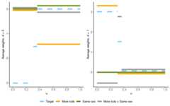
avg1<-NULL## The data.frame that will contain the average weightsi<-0## An index for the type of weightfor (jinc('w1','sw1','sw2','sw3','sw4')) {    dt<-data.frame(get(j))    avg<-rbind(## Average for u in [0, pscore[1])c(s = i,d =1,lb =0,ub = pscore[1],avgWeight =mean(dt$mp)),## Average for u in [pscore[1], pscore[2])c(s = i,d =1,lb = pscore[1],ub = pscore[2],avgWeight =mean(as.integer(dt$ub==                                      pscore[2])* dt$mp)),## Average for u in [pscore[2], 1]c(s = i,d =1,lb = pscore[2],ub =1,avgWeight =0))    avg1<-rbind(avg1, avg)    i<- i+1}avg1<-data.frame(avg1)

• The first region,[0, pscore[1]), contains agents whotake up treatment regardless of whethersamesex = FALSE orsamesex = TRUE. The average weight can therefore beestimated simply by taking the average of the weights assigned to eachagent.
• The second region,[pscore[1], pscore[2]), containsagents who would take up treatment ifsamesex = TRUE, butwould not take up treatment ifsamesex = FALSE. The weightsfor agents withsamesex = FALSE are thus 0 is in thisregion.
• Finally, the third region[pscore[2], 1], containsagents who will not take up treatment regardless of the value ofsamesex. Since the object of interest is the weights of thetreated agents, the average weight in this third region is necessarily0.

Thedata.frame created above that will be used togenerate the plot for the average treated weights takes on the followingform.

• The first column indicates the type of weight. A value of0 indicates the weight corresponds to the target parameter.Integers greater than 0 indicate the weight corresponds to the IV-likeestimand with the same index.
• The second column indicates that the weights above correspond to thetreated agents.
• The third and fourth columns indicate the region in the unitinterval that the average weights correspond to.
• The final column contains the average weights.

Adjusting for overlaps, the table above generates the plot below onthe right. The analogous table containing the average untreated weightsgenerates the plot on the left. For clarity, the weights for associatedwith the intercept have been omitted from both plots.

Help, Feature Requestsand Bug Reports

Please post an issue on theGitHubrepository.

References