


![]()
qtl2pleio is a software package for use with theR statistical computingenvironment.qtl2pleio is freely available for downloadand use. I share it under theMIT license.The user will also want to download and install theqtl2 R package.
Clickhereto exploreqtl2pleio within a liveRstudio session in “the cloud”.
We eagerly welcome contributions toqtl2pleio. All pullrequests will be considered. Features requests and bug reports may befiled as Github issues. All contributors must abide by thecodeof conduct.
For technical support, please open a Github issue. If you’re justgetting started withqtl2pleio, please examine thevignettes on thepackage’s web site. Youcan also emailfrederick.boehm@gmail.comfor assistance.
The goal ofqtl2pleio is, for a pair of traits that showevidence for a QTL in a common region, to distinguish between pleiotropy(the null hypothesis, that they are affected by a common QTL) and thealternative that they are affected by separate QTL. It extends thelikelihood ratio test ofJiang and Zeng(1995) for multiparental populations, such as Diversity Outbredmice, including the use of multivariate polygenic random effects toaccount for population structure.qtl2pleio data structuresare those used in therqtl/qtl2 package.
To install qtl2pleio, useinstall_github() from thedevtools package.
install.packages("qtl2pleio")You may also wish to install theR/qtl2. We will use it below.
install.packages("qtl2")Below, we walk through an example analysis with Diversity Outbredmouse data. We need a number of preliminary steps before we can performour test of pleiotropy vs. separate QTL. Many procedures rely on the Rpackageqtl2. We first load theqtl2 andqtl2pleio packages.
library(qtl2)library(qtl2pleio)library(ggplot2)qtl2data repository on githubWe’ll consider theDOexdata in theqtl2datarepository. We’ll download the DOex.zip file before calculating founderallele dosages.
file<-paste0("https://raw.githubusercontent.com/rqtl/","qtl2data/master/DOex/DOex.zip")DOex<-read_cross2(file)probs<-calc_genoprob(DOex)Let’s calculate the founder allele dosages from the 36-state genotypeprobabilities.
pr<-genoprob_to_alleleprob(probs)We now have an allele probabilities object stored inpr.
names(pr)#> [1] "2" "3" "X"dim(pr$`2`)#> [1] 261 8 127We see thatpr is a list of 3 three-dimensional arrays -one array for each of 3 chromosomes.
For our statistical model, we need a kinship matrix. We get one withthecalc_kinship function in therqtl/qtl2package.
kinship<-calc_kinship(probs = pr,type ="loco")We use the multivariate linear mixed effects model:
[vec(Y) = X vec(B) + vec(G) + vec(E)]
where (Y) contains phenotypes, X contains founder alleleprobabilities and covariates, and B contains founder allele effects. Gis the polygenic random effects, while E is the random errors. Weprovide more details in the vignette.
qtl2pleio::sim1The function to simulate phenotypes inqtl2pleio issim1.
# set up the design matrix, Xpp<- pr[[2]]#we'll work with Chr 3's genotype data#Next, we prepare a design matrix XX<- gemma2::stagger_mats(pp[ , ,50], pp[ , ,50])# assemble B matrix of allele effectsB<-matrix(data =c(-1,-1,-1,-1,1,1,1,1,-1,-1,-1,-1,1,1,1,1),nrow =8,ncol =2,byrow =FALSE)# set.seed to ensure reproducibilityset.seed(2018-01-30)Sig<-calc_Sigma(Vg =diag(2),Ve =diag(2),kinship = kinship[[2]])# call to sim1Ypre<-sim1(X = X,B = B,Sigma = Sig)Y<-matrix(Ypre,nrow =261,ncol =2,byrow =FALSE)rownames(Y)<-rownames(pp)colnames(Y)<-c("tr1","tr2")Let’s perform univariate QTL mapping for each of the two traits inthe Y matrix.
s1<-scan1(genoprobs = pr,pheno = Y,kinship = kinship)Here is a plot of the results.

And here are the observed QTL peaks with LOD > 8.
find_peaks(s1,map = DOex$pmap,threshold=8)#> lodindex lodcolumn chr pos lod#> 1 1 tr1 3 82.77806 20.703383#> 2 2 tr2 3 82.77806 14.417924#> 3 2 tr2 X 48.10040 8.231551We now have the inputs that we need to do a pleiotropy vs. separateQTL test. We have the founder allele dosages for one chromosome,i.e., Chr 3, in the R objectpp, the matrix of twotrait measurements inY, and a LOCO-derived kinship matrix,kinship[[2]].
out<-suppressMessages(scan_pvl(probs = pp,pheno = Y,kinship = kinship[[2]],# 2nd entry in kinship list is Chr 3start_snp =38,n_snp =25 ))To visualize results from our two-dimensional scan, we calculateprofile LOD for each trait. The code below makes use of the R packageggplot2 to plot profile LODs over the scan region.
library(dplyr)out%>%calc_profile_lods()%>%add_pmap(pmap = DOex$pmap$`3`)%>%ggplot()+geom_line(aes(x = marker_position,y = profile_lod,colour = trait))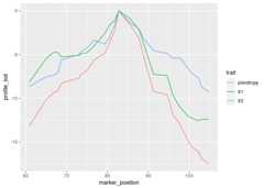
We use the functioncalc_lrt_tib to calculate thelikelihood ratio test statistic value for the specified traits andspecified genomic region.
(lrt<-calc_lrt_tib(out))#> [1] 0Before we callboot_pvl, we need to identify the index(on the chromosome under study) of the marker that maximizes thelikelihood under the pleiotropy constraint. To do this, we use theqtl2pleio functionfind_pleio_peak_tib.
(pleio_index<-find_pleio_peak_tib(out,start_snp =38))#> log10lik13#> 50set.seed(2018-11-25)# set for reproducibility purposes.b_out<-suppressMessages(boot_pvl(probs = pp,pheno = Y,pleio_peak_index = pleio_index,kinship = kinship[[2]],# 2nd element in kinship list is Chr 3nboot =10,start_snp =38,n_snp =25 ))(pvalue<-mean(b_out>= lrt))#> [1] 1citation("qtl2pleio")#>#> To cite qtl2pleio in publications use:#>#> Boehm FJ, Chesler EJ, Yandell BS, Broman KW (2019) Testing pleiotropy#> vs. separate QTL in multiparental populations G3#> https://www.g3journal.org/content/9/7/2317#>#> A BibTeX entry for LaTeX users is#>#> @Article{Boehm2019testing,#> title = {Testing pleiotropy vs. separate QTL in multiparental populations},#> author = {Frederick J. Boehm and Elissa J. Chesler and Brian S. Yandell and Karl W. Broman},#> journal = {G3},#> year = {2019},#> volume = {9},#> issue = {7},#> url = {https://www.g3journal.org/content/9/7/2317},#> eprint = {https://www.g3journal.org/content/ggg/9/7/2317.full.pdf},#> }