

The goal of ‘midr’ is to provide a model-agnostic method forinterpreting and explaining black-box predictive models by creating aglobally interpretable surrogate model. The package implements ‘MaximumInterpretation Decomposition’ (MID), a functional decompositiontechnique that finds an optimal additive approximation of the originalmodel. This approximation is achieved by minimizing the squared errorbetween the predictions of the black-box model and the surrogate model.The theoretical foundations of MID are described in Iwasawa &Matsumori (2025) [Forthcoming], and the package itself is detailed inAsashiba et al. (2025).
You can install the released version of midr fromCRAN with:
install.packages("midr")and the development version fromGitHub with:
# install.packages("devtools")devtools::install_github("ryo-asashi/midr")In the following example, we fit a random forest model to theBoston dataset included in ISLR2, and then attempt tointerpret it using the functions of midr.
# load required packageslibrary(midr)library(ggplot2)library(gridExtra)library(ISLR2)library(ranger)theme_set(theme_midr())# split the Boston datasetdata("Boston",package ="ISLR2")set.seed(42)idx<-sample(nrow(Boston),nrow(Boston)* .75)train<- Boston[ idx, ]valid<- Boston[-idx, ]# fit a random forest modelrf<-ranger(medv~ ., train,mtry =5)preds_rf<-predict(rf, valid)$predictionscat("RMSE: ",weighted.loss(valid$medv, preds_rf))#> RMSE: 3.351362The first step is to create a MID model as a global surrogate of thetarget model usinginterpret().
# fit a two-dimensional MID modelmid<-interpret(medv~ .^2, train, rf,lambda = .1)mid#>#> Call:#> interpret(formula = yhat ~ .^2, data = train, model = rf, lambda = 0.1)#>#> Model Class: ranger#>#> Intercept: 22.446#>#> Main Effects:#> 12 main effect terms#>#> Interactions:#> 66 interaction terms#>#> Uninterpreted Variation Ratio: 0.016249preds_mid<-predict(mid, valid)cat("RMSE: ",weighted.loss(preds_rf, preds_mid))#> RMSE: 1.106763cat("RMSE: ",weighted.loss(valid$medv, preds_mid))#> RMSE: 3.306072To visualize the main and interaction effects of the variables, applyggmid() orplot() to the fitted MID model.
# visualize the main and interaction effects of the MID modelgrid.arrange(ggmid(mid,"lstat")+ggtitle("main effect of lstat"),ggmid(mid,"dis")+ggtitle("main effect of dis"),ggmid(mid,"lstat:dis")+ggtitle("interaction of lstat:dis"),ggmid(mid,"lstat:dis",main.effects =TRUE,type ="compound")+ggtitle("interaction + main effects"))
# visualize all main effectsgrid.arrange(grobs =mid.plots(mid),nrow =3)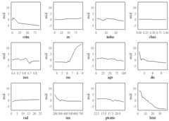
mid.importance() helps to compute and compare theimportance of main and interaction effects.
# visualize the MID importance of the component functionsimp<-mid.importance(mid)grid.arrange(nrow = 1L,ggmid(imp,"dotchart",theme ="highlight")+theme(legend.position ="bottom")+ggtitle("importance of variable effects"),ggmid(imp,"heatmap")+theme(legend.position ="bottom")+ggtitle("heatmap of variable importance"))
mid.breakdown() provides a way to analyze individualpredictions by decomposing the differences between the intercept and thepredicted value into variable effects.
# visualize the MID breakdown of the model predictionsbd1<-mid.breakdown(mid,data = train,row = 1L)bd9<-mid.breakdown(mid,data = train,row = 9L)grid.arrange(nrow = 1L,ggmid(bd1,"waterfall",theme ="midr",max.nterms = 14L)+theme(legend.position ="bottom")+ggtitle("breakdown of prediction 1"),ggmid(bd9,"waterfall",theme ="midr",max.nterms = 14L)+theme(legend.position ="bottom")+ggtitle("breakdown of prediction 9"))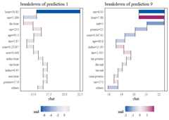
mid.conditional() can be used to compute the ICE curves(Goldstein et al. 2015) of the fitted MID model, as well as thebreakdown of the ICE curves by main and interaction effects.
# visualize the ICE curves of the MID modelice<-mid.conditional(mid,"lstat")grid.arrange(ggmid(ice,alpha = .1)+ggtitle("ICE of lstat"),ggmid(ice,"centered","mako",var.color = dis)+ggtitle("c-ICE of lstat"),ggmid(ice,term ="lstat:dis",theme ="mako",var.color = dis)+ggtitle("ICE of interaction with dis"),ggmid(ice,term ="lstat:age",theme ="mako",var.color = age)+ggtitle("ICE of interaction with age"))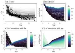
[1] Iwasawa, H. & Matsumori, Y. (2025). “A FunctionalDecomposition Approach to Maximize the Interpretability of Black-BoxModels”. [Forthcoming]
[2] Asashiba, R., Kozuma, R. & Iwasawa, H. (2025). “midr:Learning from Black-Box Models by Maximum Interpretation Decomposition”.https://arxiv.org/abs/2506.08338
[3] Goldstein, A., Kapelner, A., Bleich, J., & Pitkin, E. (2015).“Peeking Inside the Black Box: Visualizing Statistical Learning WithPlots of Individual Conditional Expectation”. Journal ofComputational and Graphical Statistics, 24(1), 44–65.https://doi.org/10.1080/10618600.2014.907095