Movatterモバイル変換

Algorithmic tesselationwith geogrid

Joseph Bailey 2023-08-15

geogrid

Turn geospatial polygons like states, counties or local authoritiesinto regular or hexagonal grids automatically.

Intro

Using geospatial polygons to portray geographical information can bea challenge when polygons are of different sizes. For example, it can bedifficult to ensure that larger polygons do not skew how readers retainor absorb information. As a result, many opt to generate maps that useconsistent shapes (i.e. regular grids) to ensure that no specificgeography is emphasised unfairly. Generally there are four reasons thatone might transform geospatial polygons to a different grid (orgeospatial representation):

1. We may use cartograms to represent the number of people (or anyvalue) within a particular geography. For more information and examplesseehereandhere.This cartogram approach changes the size of a particular geographyin-line with the values that one seeks to visualise.
2. We may use grids to bin data and typically visualise the spatialdensity of a particular variable. For an example seehere.
3. We may use grids to segment a geographical region. For exampletesselation can be used inbiologicalsampling or even in generatinggameenvironments.
4. We may use grids to ‘fairly’ represent existing geographicalentities (such as US states, UK local authorities, or even countries inEurope). For an example of representing US states as both regular andhexagonal grids seehere.

The link in bullet 4 provides an excellent introduction to the notionof tesselation and its challenges. Interestingly, the eventualgeneration of hexagonal and regular grids demonstrated in the articlewas donemanually. I believe that this can be very timeconsuming, and though it may stimulate some fun discussion - wouldn’t itbe great to do it automatically?

Recent functionality for representing US states, European countriesand World countries in a grid has been made available for ggplot2here and there are manyother great examples ofhand-specified orbespoke grids. The challenge with this is that if youhave a less commonly used geography then it might be hard to find ahand-specified orbespoke grid foryour area of interest.

What I wanted to do withgeogrid is make it easier togenerate these grids in ways that might be visually appealing and thenassign the original geographies to their gridded counterparts in a waythat made sense. Using an input of geospatial polgyonsgeogrid will generate either a regular or hexagonal grid,and then assign each of the polygons in your original file to that newgrid.

Idea

There are two steps to usinggeogrid:

1. Generate a regular or hexagonal grid of your choice. There are lotsof different arrangements of these grids so choosing one with thecalculate_grid function and varying theseedis a good place to start.
2. Use thehungarianalgorithm to efficiently calculate the assignments from theoriginal geography to the new geography. This involves identifying thesolution where the total distance between the centroid of every originalgeography and its new centroid on the grid is minimised. For this I haveincluded a previous implementation of the Hungarian algorithm kindlymade availablehere.Huge thanks to Lars Simon Zehnder for this implementation.

Example

This is a basic example which shows how the assignment of Londonboroughs could work.

library(geogrid)library(sf)library(tmap)input_file<-system.file("extdata","london_LA.json",package ="geogrid")original_shapes<-st_read(input_file)%>%st_set_crs(27700)original_shapes$SNAME<-substr(original_shapes$NAME,1,4)

For reference, lets see how London’s local authorities are actuallybounded in real space. In this example, I have coloured each polygonbased on it’s area. Brighter polygons are larger.

rawplot<-tm_shape(original_shapes)+tm_polygons("HECTARES",palette ="viridis")+tm_text("SNAME")rawplot

So, let’s turn this into a grid to stop places like Bromley,Hillingdon and Havering from stealing our attention. First of all, wecan generate a number of different grids usingseed. Sincethere are many ways to dissect the outer boundary of the polygons youmight want to choose an output that appeals to you. I’d recommendlooking at differentseed values and choosing the one thatbest matches the outline that you approve of.

Thecalculate_grid function takes in aSpatialPolygonsDataframe or sf object, a learning rate (suggestion =0.03 to begin), a grid typehexagonal orregular and a seed value. Let’s have a look at somehexagonal grid options for the London local authorities:

par(mfrow =c(2,3),mar =c(0,0,2,0))for (iin1:6) {  new_cells<-calculate_grid(shape = original_shapes,grid_type ="hexagonal",seed = i)plot(new_cells,main =paste("Seed", i,sep =" "))}

Let’s also look at things with a regular grid:

par(mfrow =c(2,3),mar =c(0,0,2,0))for (iin1:6) {  new_cells<-calculate_grid(shape = original_shapes,grid_type ="regular",seed = i)plot(new_cells,main =paste("Seed", i,sep =" "))}

As we can see there are lots of options. Now, lets choose a grid andassign our existing places to it. I happen to like the both grids thathave aseed of 3. So I’m going to assign the polygons tothose grids. Let’s do that and see what they look like compared to theoriginal.

new_cells_hex<-calculate_grid(shape = original_shapes,grid_type ="hexagonal",seed =3)resulthex<-assign_polygons(original_shapes, new_cells_hex)new_cells_reg<-calculate_grid(shape = original_shapes,grid_type ="regular",seed =3)resultreg<-assign_polygons(original_shapes, new_cells_reg)

Now we have an example transfer from real space to grid space - wecan visualise it.

hexplot<-tm_shape(resulthex)+tm_polygons("HECTARES",palette ="viridis")+tm_text("SNAME")regplot<-tm_shape(resultreg)+tm_polygons("HECTARES",palette ="viridis")+tm_text("SNAME")tmap_arrange(rawplot, hexplot, regplot,nrow =3)

Details

The package has two major functions:

1. calculate_grid() given your input polygons this willgenerate the grid as specified by your arguments:
   • shape: the original polygons
   • learning_rate: the rate at which the gradient descentfinds the optimum cellsize to ensure that your gridded points fit withinthe outer boundary of the input polygons.
   • grid_type: eitherregular for a squaregrid orhexagonal for a hexagonal grid.
   • seed: the seed to ensure you get the same gridoutput.
2. assign_polygons(): this will assign the originalpolygons to their new locations on the grid generated incalculate_grid(). It will find the solution that minimisesthe sum of the total distance between the original polygon centroids andeventual gridded centroids. Arguments:
   • shape: the original polygons
   • new_polygons: the output (a list) fromcalculate_grid().

TODO

• Assignment may not always work - check theassign_polygons() why does it only work sometimes?
• Make it work (done I think), make it right (not yet), make it fast(not yet).
• Improve the cellsize calculation methodology.
• Get someone to answerthisstack overflow question.

Notes

This is my first attempt at a package. If it doesn’t work I’d likesuggestions for improvements and thanks in advance for providingthem!

I welcome critique and feedback. Blog post to follow.

Thanks

I read a lot of the work byHadleyWickham,Jenny Bryan,Thomas Lin Pedersen,Mara Averick andBob Rudis toname a few. But also love the R community and learn a huge amount fromR Bloggers.

Extra thanks go toRyan Hafenfor making this package publishable.

Other examples

From others:

Simon Hailstone has looked atmale life expectancy in theSouth East region of England using the package. Thanks Simon forusing!

From me:

This time using the contiguous USA. Again, I used set seed and chosesome that I liked but I’d recommend you’d do the same.

input_file2<-system.file("extdata","states.json",package ="geogrid")original_shapes2<-st_read(input_file2)%>%st_transform(2163)original_shapes2$SNAME<-substr(original_shapes2$NAME,1,4)rawplot2<-tm_shape(original_shapes2)+tm_polygons("CENSUSAREA",palette ="viridis")+tm_text("SNAME")

Let’s check the seeds again.

par(mfrow =c(2,3),mar =c(0,0,2,0))for (iin1:6) {  new_cells<-calculate_grid(shape = original_shapes2,grid_type ="hexagonal",seed = i)plot(new_cells,main =paste("Seed", i,sep =" "))}

par(mfrow =c(2,3),mar =c(0,0,2,0))for (iin1:6) {  new_cells<-calculate_grid(shape = original_shapes2,grid_type ="regular",seed = i)plot(new_cells,main =paste("Seed", i,sep =" "))}

Now we’ve seen some seed demo’s lets assign them…

new_cells_hex2<-calculate_grid(shape = original_shapes2,grid_type ="hexagonal",seed =6)resulthex2<-assign_polygons(original_shapes2, new_cells_hex2)new_cells_reg2<-calculate_grid(shape = original_shapes2,grid_type ="regular",seed =4)resultreg2<-assign_polygons(original_shapes2, new_cells_reg2)hexplot2<-tm_shape(resulthex2)+tm_polygons("CENSUSAREA",palette ="viridis")+tm_text("SNAME")regplot2<-tm_shape(resultreg2)+tm_polygons("CENSUSAREA",palette ="viridis")+tm_text("SNAME")tmap_arrange(rawplot2, hexplot2, regplot2,nrow =3)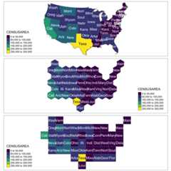

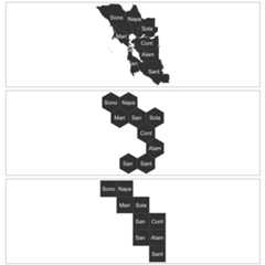
Likewise, you can try the bay area…

input_file3<-system.file("extdata","bay_counties.geojson",package ="geogrid")original_shapes3<-st_read(input_file3)%>%st_transform(3310)original_shapes3$SNAME<-substr(original_shapes3$county,1,4)rawplot3<-tm_shape(original_shapes3)+tm_polygons(col ="gray25")+tm_text("SNAME")new_cells_hex3<-calculate_grid(shape = original_shapes3,grid_type ="hexagonal",seed =6)resulthex3<-assign_polygons(original_shapes3, new_cells_hex3)new_cells_reg3<-calculate_grid(shape = original_shapes3,grid_type ="regular",seed =1)resultreg3<-assign_polygons(original_shapes3, new_cells_reg3)hexplot3<-tm_shape(resulthex3)+tm_polygons(col ="gray25")+tm_text("SNAME")regplot3<-tm_shape(resultreg3)+tm_polygons(col ="gray25")+tm_text("SNAME")tmap_arrange(rawplot3, hexplot3, regplot3,nrow =3)