

Package:cbbinom0.2.0
Author: Xiurui Zhu
Modified: 2024-09-18 23:27:13
Compiled: 2024-10-16 23:21:42
The goal ofcbbinom is to implement continuousbeta-binomial distribution.
You can install the released version ofcbbinom fromCRAN with:
install.packages("cbbinom")Alternatively, you can install the developmental version ofcbbinom fromgithubwith:
remotes::install_github("zhuxr11/cbbinom")The continuous beta-binomial distribution spreads the standardprobability mass of beta-binomial distribution atx to aninterval[x, x + 1] in a continuous manner. This can bevalidated via the following plot, where we can see that the cumulativedistribution function (CDF) of the continuous beta-binomial distributionatx + 1 equals to that of the beta-binomial distributionatx.
library(cbbinom)# The continuous beta-binomial CDF, shift by -1cbbinom_plot_x<-seq(-1,10,0.01)cbbinom_plot_y<-pcbbinom(q = cbbinom_plot_x,size =10,alpha =2,beta =4,ncp =-1)# The beta-binomial CDFbbinom_plot_x<-seq(0L, 10L, 1L)bbinom_plot_y<- extraDistr::pbbinom(q = bbinom_plot_x,size = 10L,alpha =2,beta =4)ggplot2::ggplot(mapping = ggplot2::aes(x = x,y = y))+ ggplot2::geom_bar(data =data.frame(x = bbinom_plot_x,y = bbinom_plot_y ),stat ="identity" )+ ggplot2::geom_point(data =data.frame(x = cbbinom_plot_x,y = cbbinom_plot_y ) )+ ggplot2::scale_x_continuous(n.breaks =diff(range(cbbinom_plot_x)) )+ ggplot2::theme_bw()+ ggplot2::labs(y ="CDF(x)")
However, the central density atx + 1/2 of thecontinuous beta-binomial distribution may not equal to the correspondingprobability mass atx, especially around the summit and tothe right (sincealpha < beta).
# The continuous beta-binomial CDF, shift by -1/2cbbinom_plot_x_d<-seq(-1/2,10+1/2,0.01)cbbinom_plot_y_d<-dcbbinom(x = cbbinom_plot_x_d,size =10,alpha =2,beta =4,ncp =-1/2)# The beta-binomial CDFbbinom_plot_x<-seq(0L, 10L, 1L)bbinom_plot_y_d<- extraDistr::dbbinom(x = bbinom_plot_x,size = 10L,alpha =2,beta =4)ggplot2::ggplot(mapping = ggplot2::aes(x = x,y = y))+ ggplot2::geom_bar(data =data.frame(x = bbinom_plot_x,y = bbinom_plot_y_d ),stat ="identity" )+ ggplot2::geom_point(data =data.frame(x = cbbinom_plot_x_d,y = cbbinom_plot_y_d ) )+ ggplot2::scale_x_continuous(n.breaks =diff(range(bbinom_plot_x)) )+ ggplot2::theme_bw()+ ggplot2::labs(y ="PDF(x)")
For larger sizes, you may need higher precision than double foraccuracy, at the cost of computational speed.
cbbinom_plot_prec_x_p<-seq(0,41,0.1)# Compute CDF at default (double) precision levelsystem.time(pcbbinom_plot_prec0_y<-pcbbinom(q = cbbinom_plot_prec_x_p,size =40,alpha =2,beta =4,prec =NULL))#> user system elapsed#> 0.03 0.00 0.03ggplot2::ggplot(data =data.frame(x = cbbinom_plot_prec_x_p,y = pcbbinom_plot_prec0_y),mapping = ggplot2::aes(x = x,y = y))+ ggplot2::geom_point()+ ggplot2::theme_bw()+ ggplot2::labs(y ="CDF(x)")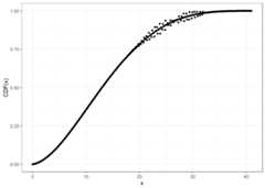
# Compute CDF at precision level 20system.time(pcbbinom_plot_prec20_y<-pcbbinom(q = cbbinom_plot_prec_x_p,size =40,alpha =2,beta =4,prec = 20L))#> user system elapsed#> 1.57 0.00 1.59ggplot2::ggplot(data =data.frame(x = cbbinom_plot_prec_x_p,y = pcbbinom_plot_prec20_y),mapping = ggplot2::aes(x = x,y = y))+ ggplot2::geom_point()+ ggplot2::theme_bw()+ ggplot2::labs(y ="CDF(x)")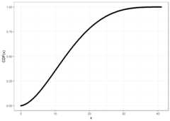
As the probability distributions instats package,cbbinom provides a full set of density, distributionfunction, quantile function and random generation for the continuousbeta-binomial distribution.
# Density functiondcbbinom(x =5,size =10,alpha =2,beta =4)#> [1] 0.12669# Distribution function(test_val<-pcbbinom(q =5,size =10,alpha =2,beta =4))#> [1] 0.7062937# Quantile functionqcbbinom(p = test_val,size =10,alpha =2,beta =4)#> [1] 5# Random generationset.seed(1111L)rcbbinom(n = 10L,size =10,alpha =2,beta =4)#> [1] 3.359039 3.038286 7.110936 1.311321 5.264688 8.709005 6.720415 1.164210#> [9] 3.868370 1.332590These functions are also available inRcpp ascbbinom::cpp_*cbbinom(), when using[[Rcpp::depends(cbbinom)]] and#include <cbbinom.h>.
For mathematical details, please check the details section of?cbbinom.
Rcppimplementation ofstats::uniroot()As a bonus,cbbinom also exports anRcppimplementation ofstats::uniroot() function, which may comein handy to solve equations, especially the monotonic ones used inquantile functions. Here is an example to calculateqnormfrompnorm inRcpp.
#include<iostream>#include"cbbinom.h"usingnamespace cbbinom;// Define a functor as pnorm() - pclass PnormEqn:public UnirootEqn{private:double mu;double sd;double p;public: PnormEqn(constdoublemu_,constdoublesd_,constdoublep_): mu(mu_), sd(sd_), p(p_){}doubleoperator()(constdouble& x)constoverride{return R::pnorm(x,this->mu,this->sd,true,false)-this->p;}};// Compute quantilesint main(){double p=0.975;// Quantile PnormEqn eqn_obj(0.0,1.0,0.975);double tol=1e-6;int max_iter=10000;double q= cbbinom::cpp_uniroot(-1000.0,1000.0,-p,1.0- p,&eqn_obj,&tol,&max_iter);std::cout <<"Quantile at "<< p<<"is: "<< q<<std::endl;return0;}