


Thebrms package provides an interface to fitBayesian generalized (non-)linear multivariate multilevel models usingStan, which is a C++ package for performing full Bayesian inference (seehttps://mc-stan.org/).The formula syntax is very similar to that of the package lme4 toprovide a familiar and simple interface for performing regressionanalyses. A wide range of response distributions are supported, allowingusers to fit – among others – linear, robust linear, count data,survival, response times, ordinal, zero-inflated, and even self-definedmixture models all in a multilevel context. Further modeling optionsinclude non-linear and smooth terms, auto-correlation structures,censored data, missing value imputation, and quite a few more. Inaddition, all parameters of the response distribution can be predictedin order to perform distributional regression. Multivariate models(i.e., models with multiple response variables) can be fit, as well.Prior specifications are flexible and explicitly encourage users toapply prior distributions that actually reflect their beliefs. Model fitcan easily be assessed and compared with posterior predictive checks,cross-validation, and Bayes factors.
library(brms)As a simple example, we use poisson regression to model the seizurecounts in epileptic patients to investigate whether the treatment(represented by variableTrt) can reduce the seizure countsand whether the effect of the treatment varies with the (standardized)baseline number of seizures a person had before treatment (variablezBase). As we have multiple observations per person, agroup-level intercept is incorporated to account for the resultingdependency in the data.
fit1<-brm(count~ zAge+ zBase* Trt+ (1|patient),data = epilepsy,family =poisson())The results (i.e., posterior draws) can be investigated using
summary(fit1)#> Family: poisson#> Links: mu = log#> Formula: count ~ zAge + zBase * Trt + (1 | patient)#> Data: epilepsy (Number of observations: 236)#> Draws: 4 chains, each with iter = 2000; warmup = 1000; thin = 1;#> total post-warmup draws = 4000#>#> Multilevel Hyperparameters:#> ~patient (Number of levels: 59)#> Estimate Est.Error l-95% CI u-95% CI Rhat Bulk_ESS Tail_ESS#> sd(Intercept) 0.59 0.07 0.46 0.74 1.01 566 1356#>#> Regression Coefficients:#> Estimate Est.Error l-95% CI u-95% CI Rhat Bulk_ESS Tail_ESS#> Intercept 1.78 0.12 1.55 2.01 1.00 771 1595#> zAge 0.09 0.09 -0.08 0.27 1.00 590 1302#> zBase 0.71 0.12 0.47 0.96 1.00 848 1258#> Trt1 -0.27 0.16 -0.60 0.05 1.01 749 1172#> zBase:Trt1 0.05 0.17 -0.30 0.38 1.00 833 1335#>#> Draws were sampled using sampling(NUTS). For each parameter, Bulk_ESS#> and Tail_ESS are effective sample size measures, and Rhat is the potential#> scale reduction factor on split chains (at convergence, Rhat = 1).On the top of the output, some general information on the model isgiven, such as family, formula, number of iterations and chains. Next,group-level effects are displayed separately for each grouping factor interms of standard deviations and (in case of more than one group-leveleffect per grouping factor; not displayed here) correlations betweengroup-level effects. On the bottom of the output, population-leveleffects (i.e. regression coefficients) are displayed. If incorporated,autocorrelation effects and family specific parameters (e.g., theresidual standard deviation ‘sigma’ in normal models) are alsogiven.
In general, every parameter is summarized using the mean (‘Estimate’)and the standard deviation (‘Est.Error’) of the posterior distributionas well as two-sided 95% credible intervals (‘l-95% CI’ and ‘u-95% CI’)based on quantiles. We see that the coefficient ofTrt isnegative with a zero overlapping 95%-CI. This indicates that, onaverage, the treatment may reduce seizure counts by some amount but theevidence based on the data and applied model is not very strong andstill insufficient by standard decision rules. Further, we find littleevidence that the treatment effect varies with the baseline number ofseizures.
The last three values (‘ESS_bulk’, ‘ESS_tail’, and ‘Rhat’) provideinformation on how well the algorithm could estimate the posteriordistribution of this parameter. If ‘Rhat’ is considerably greater than1, the algorithm has not yet converged and it is necessary to run moreiterations and / or set stronger priors.
To visually investigate the chains as well as the posteriordistributions, we can use theplot method. If we just wantto see results of the regression coefficients ofTrt andzBase, we go for
plot(fit1,variable =c("b_Trt1","b_zBase"))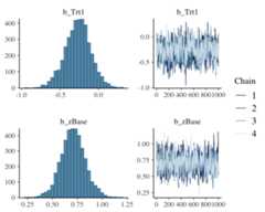
A more detailed investigation can be performed by runninglaunch_shinystan(fit1). To better understand therelationship of the predictors with the response, I recommend theconditional_effects method:
plot(conditional_effects(fit1,effects ="zBase:Trt"))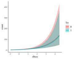
This method uses some prediction functionality behind the scenes,which can also be called directly. Suppose that we want to predictresponses (i.e. seizure counts) of a person in the treatment group(Trt = 1) and in the control group (Trt = 0)with average age and average number of previous seizures. Than we canuse
newdata<-data.frame(Trt =c(0,1),zAge =0,zBase =0)predict(fit1,newdata = newdata,re_formula =NA)#> Estimate Est.Error Q2.5 Q97.5#> [1,] 5.91200 2.494857 2 11#> [2,] 4.57325 2.166058 1 9We need to setre_formula = NA in order not to conditionof the group-level effects. While thepredict methodreturns predictions of the responses, thefitted methodreturns predictions of the regression line.
fitted(fit1,newdata = newdata,re_formula =NA)#> Estimate Est.Error Q2.5 Q97.5#> [1,] 5.945276 0.7075160 4.696257 7.450011#> [2,] 4.540081 0.5343471 3.579757 5.665132Both methods return the same estimate (up to random error), while thelatter has smaller variance, because the uncertainty in the regressionline is smaller than the uncertainty in each response. If we want topredict values of the original data, we can just leave thenewdata argument empty.
Suppose, we want to investigate whether there is overdispersion inthe model, that is residual variation not accounted for by the responsedistribution. For this purpose, we include a second group-levelintercept that captures possible overdispersion.
fit2<-brm(count~ zAge+ zBase* Trt+ (1|patient)+ (1|obs),data = epilepsy,family =poisson())We can then go ahead and compare both models via approximateleave-one-out (LOO) cross-validation.
loo(fit1, fit2)#> Output of model 'fit1':#>#> Computed from 4000 by 236 log-likelihood matrix.#>#> Estimate SE#> elpd_loo -671.7 36.6#> p_loo 94.3 14.2#> looic 1343.4 73.2#> ------#> MCSE of elpd_loo is NA.#> MCSE and ESS estimates assume MCMC draws (r_eff in [0.4, 2.0]).#>#> Pareto k diagnostic values:#> Count Pct. Min. ESS#> (-Inf, 0.7] (good) 228 96.6% 157#> (0.7, 1] (bad) 7 3.0% <NA>#> (1, Inf) (very bad) 1 0.4% <NA>#> See help('pareto-k-diagnostic') for details.#>#> Output of model 'fit2':#>#> Computed from 4000 by 236 log-likelihood matrix.#>#> Estimate SE#> elpd_loo -596.8 14.0#> p_loo 109.7 7.2#> looic 1193.6 28.1#> ------#> MCSE of elpd_loo is NA.#> MCSE and ESS estimates assume MCMC draws (r_eff in [0.4, 1.7]).#>#> Pareto k diagnostic values:#> Count Pct. Min. ESS#> (-Inf, 0.7] (good) 172 72.9% 83#> (0.7, 1] (bad) 56 23.7% <NA>#> (1, Inf) (very bad) 8 3.4% <NA>#> See help('pareto-k-diagnostic') for details.#>#> Model comparisons:#> elpd_diff se_diff#> fit2 0.0 0.0#> fit1 -74.9 27.2Theloo output when comparing models is a littleverbose. We first see the individual LOO summaries of the two models andthen the comparison between them. Since higherelpd (i.e.,expected log posterior density) values indicate better fit, we see thatthe model accounting for overdispersion (i.e.,fit2) fitssubstantially better. However, we also see in the individual LOO outputsthat there are several problematic observations for which theapproximations may have not have been very accurate. To deal with thisappropriately, we need to fall back to other methods such asreloo orkfold but this requires the model tobe refit several times which takes too long for the purpose of a quickexample. The post-processing methods we have shown above are just thetip of the iceberg. For a full list of methods to apply on fitted modelobjects, typemethods(class = "brmsfit").
Developing and maintaining open source software is an important yetoften underappreciated contribution to scientific progress. Thus,whenever you are using open source software (or software in general),please make sure to cite it appropriately so that developers get creditfor their work.
When using brms, please cite one or more of the followingpublications:
As brms is a high-level interface to Stan, please additionally citeStan (see alsohttps://mc-stan.org/users/citations/):
Further, brms relies on several other R packages and, of course, on Ritself. To find out how to cite R and its packages, use thecitation function. There are some features of brms whichspecifically rely on certain packages. Therstanpackage together withRcpp makes Stan convenientlyaccessible in R. Visualizations and posterior-predictive checks arebased onbayesplot andggplot2.Approximate leave-one-out cross-validation usingloo andrelated methods is done via theloo package. Marginallikelihood based methods such asbayes_factor are realizedby means of thebridgesampling package. Splinesspecified via thes andt2 functions rely onmgcv. If you use some of these features, please alsoconsider citing the related packages.
To install the latest release version from CRAN use
install.packages("brms")The current developmental version can be downloaded from GitHubvia
if (!requireNamespace("remotes")) {install.packages("remotes")}remotes::install_github("paul-buerkner/brms")Because brms is based on Stan, a C++ compiler is required. Theprogram Rtools (available onhttps://cran.r-project.org/bin/windows/Rtools/) comeswith a C++ compiler for Windows. On Mac, you should install Xcode. Forfurther instructions on how to get the compilers running, see theprerequisites section onhttps://github.com/stan-dev/rstan/wiki/RStan-Getting-Started.
Detailed instructions and case studies are given in the package’sextensive vignettes. Seevignette(package = "brms") for anoverview. For documentation on formula syntax, families, and priordistributions seehelp("brm").
Questions can be asked on theStan forums on Discourse. Topropose a new feature or report a bug, please open an issue onGitHub.
If you have already fitted a model, apply thestancodemethod on the fitted model object. If you just want to generate the Stancode without any model fitting, use thestancode method onyour model formula.
When you fit your model for the first time with brms, there iscurrently no way to avoid compilation. However, if you have alreadyfitted your model and want to run it again, for instance with moredraws, you can do this without recompilation by using theupdate method. For more details seehelp("update.brmsfit").
The rstanarm package is similar to brms in that it also allows to fitregression models using Stan for the backend estimation. Contrary tobrms, rstanarm comes with precompiled code to save the compilation time(and the need for a C++ compiler) when fitting a model. However, as brmsgenerates its Stan code on the fly, it offers much more flexibility inmodel specification than rstanarm. Also, multilevel models are currentlyfitted a bit more efficiently in brms. For detailed comparisons of brmswith other common R packages implementing multilevel models, seevignette("brms_multilevel") andvignette("brms_overview").