

The goal ofbigtime is to sparsely estimate large timeseries models such as the Vector AutoRegressive (VAR) Model, the VectorAutoRegressive with Exogenous Variables (VARX) Model, and the VectorAutoRegressive Moving Average (VARMA) Model. The univariate cases arealso supported.
The package can be installed from CRAN using
install.packages("bigtime")You can install the development version (= the latest version) ofbigtime from github as follows:
# install.packages("devtools")devtools::install_github("ineswilms/bigtime")bigtime comes with example data sets created from a VAR, VARMA andVARX DGP. These data sets are calledvar.example,varma.example, andvarx.example respectivelyand can be loaded into the environment by callingdata(var.example) and similarly for the others. We can havea look at thevarx.example data set by first loading itinto the environment and then, using a little utility function, plottingit.
library(bigtime)suppressMessages(library(tidyverse))# Will be used for nicer visualisations#> Warning: package 'tidyverse' was built under R version 4.0.5#> Warning: package 'ggplot2' was built under R version 4.0.3#> Warning: package 'readr' was built under R version 4.0.4#> Warning: package 'purrr' was built under R version 4.0.3#> Warning: package 'dplyr' was built under R version 4.0.5#> Warning: package 'stringr' was built under R version 4.0.3#> Warning: package 'forcats' was built under R version 4.0.4data(varx.example)# loading the varx example dataplot_series<-function(Y){as_tibble(Y)%>%mutate(Time =1:n())%>%pivot_longer(-Time,names_to ="Series",values_to ="vals")%>%mutate(Series =factor(Series,levels =colnames(Y)))%>%ggplot()+geom_line(aes(Time, vals))+facet_wrap(facets =vars(Series),ncol =1)+ylab("")+theme_bw()}plot_series(Y.varx)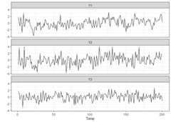
plot_series(X.varx)
While we could use the example data provided,bigtime alsosupports simulation of VAR models using both lasso and elementwise typesparsity patterns. Since lasso is the most widely known one, we willstart off with lasso. To simulate a VAR model having lasso type ofsparsity, use thesimVAR function and setsparsity_pattern="lasso". The lasso sparsity pattern hasthe additionalnum_zero option which determines the numberof zeros in the VAR coefficient matrix (excluding intercepts).Note:we also set a seed so that the simulation is replicable. We canthen use thesummary function to obtain a summary of thesimulated data.
periods<-200# time series lengthk<-5# number of time seriesp<-8# maximum lagsparsity_options<-list(num_zero =15)# 15 zeros across the k=5 VAR coefficient matricessim_data<-simVAR(periods = periods,k = k,p = p,sparsity_pattern ="lasso",sparsity_options = sparsity_options,seed =123456,decay =0.01)# the smaller decay the larger early coefs w.r.t. to later onesY.lasso<- sim_data$Ysummary(sim_data)# obtaining a summary of the simulated time series data#> #### General Information #####>#> Seed 123456#> Time series length 200#> Burnin 200#> Variables Simulated 5#> Number of Lags 8#> Coefficients were randomly created? TRUE#> Maximum Eigenvalue of Companion Matrix 0.8#> Sparsity Pattern lasso#>#>#> #### Sparsity Options #####>#> $num_zero#> [1] 15#>#>#>#> #### Coefficient Matrix #####>#> Y1 Y2 Y3 Y4 Y5#> Y1.L1 3.344178e-01 -1.107252e-01 -1.423944e-01 3.509198e-02 9.033998e-01#> Y2.L1 3.347094e-01 5.264215e-01 1.003833e+00 4.685881e-01 -1.709388e-01#> Y3.L1 -3.995565e-01 -4.468152e-01 -2.235442e-02 4.710753e-01 4.224553e-01#> Y4.L1 2.310627e-02 -2.948322e-01 3.732432e-01 6.691342e-01 2.244958e-01#> Y5.L1 0.000000e+00 5.040150e-01 1.543970e-02 7.602611e-02 1.855509e-01#> Y1.L2 -1.714191e-03 6.652793e-05 2.827333e-03 3.898174e-03 -2.488847e-03#> Y2.L2 -3.432958e-03 2.790046e-04 -4.196394e-03 -1.102596e-02 -4.531967e-03#> Y3.L2 -3.456294e-03 6.257595e-03 4.071610e-03 4.187554e-03 -4.475995e-03#> Y4.L2 0.000000e+00 3.882016e-03 6.860267e-04 -3.594939e-03 6.349122e-04#> Y5.L2 -2.013360e-03 0.000000e+00 -4.561977e-04 4.355841e-03 -4.860029e-03#> Y1.L3 -7.090490e-05 -1.972221e-05 1.289428e-05 0.000000e+00 0.000000e+00#> Y2.L3 -1.362040e-05 -4.321743e-05 -5.979591e-05 -1.013789e-05 -4.890420e-06#> Y3.L3 -2.603130e-05 1.255775e-05 4.926041e-06 -3.356641e-05 2.408345e-05#> Y4.L3 -9.864658e-06 -7.407063e-06 9.288386e-07 -1.943981e-05 -2.959808e-05#> Y5.L3 5.224473e-05 2.264257e-05 -7.240193e-05 1.758216e-05 -5.780336e-05#> Y1.L4 3.821882e-07 -2.899947e-07 1.955819e-08 -6.271466e-07 -9.234996e-07#> Y2.L4 4.644695e-07 -2.826756e-07 -6.312740e-07 2.079154e-07 -4.271531e-07#> Y3.L4 1.887393e-08 3.401594e-07 1.735509e-07 2.097019e-07 0.000000e+00#> Y4.L4 -1.992917e-07 5.054378e-07 2.266186e-07 -1.382372e-07 2.907276e-07#> Y5.L4 3.465950e-07 1.481081e-07 6.351945e-07 2.421511e-08 5.162710e-08#> Y1.L5 -3.412591e-09 4.406386e-09 -4.838797e-09 2.333901e-09 3.464337e-09#> Y2.L5 3.943109e-09 -5.099138e-09 -4.262808e-12 -3.854296e-09 5.050800e-09#> Y3.L5 -3.476037e-09 9.989383e-10 -3.456284e-10 -1.977003e-09 -1.078979e-09#> Y4.L5 -1.601388e-09 -3.787661e-09 4.063988e-09 -1.639348e-09 -7.263552e-10#> Y5.L5 4.748150e-09 -6.451814e-09 -9.114958e-09 -8.185059e-09 -2.599211e-09#> Y1.L6 2.878848e-11 -4.147466e-12 0.000000e+00 -3.921230e-11 0.000000e+00#> Y2.L6 1.757755e-12 -4.097641e-11 3.182509e-11 2.012060e-11 -6.235119e-11#> Y3.L6 3.543788e-11 -8.333751e-12 7.345804e-11 7.110232e-12 -3.232298e-11#> Y4.L6 7.813330e-11 4.861321e-12 -1.423732e-11 4.223140e-11 4.665353e-11#> Y5.L6 -3.204189e-11 3.110420e-11 -8.002152e-11 -1.406136e-11 1.527682e-11#> Y1.L7 1.035718e-13 3.868736e-13 0.000000e+00 3.274603e-14 -6.488767e-14#> Y2.L7 5.105382e-13 -2.889064e-13 6.181295e-13 3.424112e-13 3.218496e-13#> Y3.L7 -1.374288e-13 4.027135e-14 6.096383e-14 0.000000e+00 -1.371909e-13#> Y4.L7 -5.274508e-13 -7.661388e-13 2.324513e-13 -6.879730e-13 0.000000e+00#> Y5.L7 -6.332500e-13 7.399670e-13 3.913858e-13 -1.324464e-13 4.786837e-13#> Y1.L8 -1.337775e-15 6.673161e-16 0.000000e+00 7.885634e-15 2.243677e-15#> Y2.L8 -2.573135e-15 -1.884193e-16 4.549152e-15 1.160132e-15 1.854712e-15#> Y3.L8 4.740580e-15 0.000000e+00 -2.501340e-15 -2.635646e-15 2.839144e-15#> Y4.L8 0.000000e+00 -1.797436e-15 4.488466e-15 7.460492e-16 -1.452254e-15#> Y5.L8 9.907469e-16 1.438249e-15 6.791980e-17 -9.437176e-16 0.000000e+00
A VAR with HLag (elementwise) type of sparsity can be simulated usingsimVAR and by settingsparsity_pattern="HLag".Three extra options exist: (1)zero_min determines theminimum number of zero coefficients of each variable in each equation,(2)zero_max determines the maximum number of zerocoefficients of each variable in each equation, and (3)zeroes_in_self is a boolean option that if TRUE, zerocoefficients of theith variable can exist in theithequation.
periods<-200k<-5# Number of time seriesp<-5# Maximum lagsparsity_options<-list(zero_min =0,zero_max =5,zeroes_in_self =TRUE)sim_data<-simVAR(periods = periods,k = k,p = p,sparsity_pattern ="HLag",sparsity_options = sparsity_options,seed =123456,decay =0.01)Y.hlag<- sim_data$Ysummary(sim_data)# Obtaining a summary of the simulation#> #### General Information #####>#> Seed 123456#> Time series length 200#> Burnin 200#> Variables Simulated 5#> Number of Lags 5#> Coefficients were randomly created? TRUE#> Maximum Eigenvalue of Companion Matrix 0.8#> Sparsity Pattern hvar#>#>#> #### Sparsity Options #####>#> $zero_min#> [1] 0#>#> $zero_max#> [1] 5#>#> $zeroes_in_self#> [1] TRUE#>#>#>#> #### Coefficient Matrix #####>#> Y1 Y2 Y3 Y4 Y5#> Y1.L1 0.000000e+00 -1.032031e-01 -1.327209e-01 3.270802e-02 8.420276e-01#> Y2.L1 3.119710e-01 4.906592e-01 9.356382e-01 4.367547e-01 -1.593261e-01#> Y3.L1 -3.724128e-01 -4.164610e-01 -2.083578e-02 4.390729e-01 3.937560e-01#> Y4.L1 2.153655e-02 -2.748029e-01 3.478871e-01 0.000000e+00 2.092447e-01#> Y5.L1 -2.818808e-01 4.697750e-01 1.439081e-02 7.086130e-02 1.729456e-01#> Y1.L2 0.000000e+00 0.000000e+00 2.635259e-03 3.633353e-03 -2.319768e-03#> Y2.L2 -3.199742e-03 2.600505e-04 0.000000e+00 -1.027691e-02 -4.224090e-03#> Y3.L2 -3.221492e-03 5.832487e-03 0.000000e+00 3.903074e-03 -4.171920e-03#> Y4.L2 0.000000e+00 3.618292e-03 6.394217e-04 0.000000e+00 5.917797e-04#> Y5.L2 -1.876583e-03 -3.611195e-03 -4.252061e-04 4.059929e-03 -4.529864e-03#> Y1.L3 0.000000e+00 0.000000e+00 1.201831e-05 0.000000e+00 5.747130e-05#> Y2.L3 -1.269510e-05 -4.028146e-05 0.000000e+00 -9.449180e-06 -4.558191e-06#> Y3.L3 -2.426287e-05 1.170464e-05 0.000000e+00 -3.128609e-05 2.244735e-05#> Y4.L3 0.000000e+00 0.000000e+00 0.000000e+00 0.000000e+00 -2.758734e-05#> Y5.L3 0.000000e+00 2.110436e-05 -6.748333e-05 1.638772e-05 -5.387651e-05#> Y1.L4 0.000000e+00 0.000000e+00 1.822951e-08 0.000000e+00 -8.607620e-07#> Y2.L4 4.329159e-07 -2.634722e-07 0.000000e+00 0.000000e+00 -3.981346e-07#> Y3.L4 0.000000e+00 3.170507e-07 0.000000e+00 1.954558e-07 -9.491777e-08#> Y4.L4 0.000000e+00 0.000000e+00 0.000000e+00 0.000000e+00 0.000000e+00#> Y5.L4 0.000000e+00 1.380464e-07 5.920428e-07 0.000000e+00 4.811983e-08#> Y1.L5 0.000000e+00 0.000000e+00 0.000000e+00 0.000000e+00 3.228988e-09#> Y2.L5 0.000000e+00 0.000000e+00 0.000000e+00 0.000000e+00 0.000000e+00#> Y3.L5 0.000000e+00 0.000000e+00 0.000000e+00 -1.842696e-09 -1.005678e-09#> Y4.L5 0.000000e+00 0.000000e+00 0.000000e+00 0.000000e+00 0.000000e+00#> Y5.L5 0.000000e+00 -6.013512e-09 -8.495736e-09 0.000000e+00 0.000000e+00
The above simulated data (and truly any other data) could then beestimated using an L1-penalty (lasso penalty) on the autoregressivecoefficients. To this end, set theVARpen argument in thesparseVAR function equal to L1.Note: it is recommendedto standardise the data. Bigtime will give a warning if the data is notstandardised but will not stop you from continuing. Settingselection="none", the default, allows us to specify thepenalization we want. Furthermore, we can predefine the maximumlag-order by changing thep argument to the desired value.However, we do not recommend this, as the bigtime will, by default,choose a maximum lag-order that is well suited in many scenarios.
VAR.L1<-sparseVAR(Y =scale(Y.lasso),# standardising the dataVARpen ="L1",# using lasso penaltyVARlseq =1.5)# Specifying the penalty to be used. selection="none" is the default.For the selection of the penalization parameter, we can either settheselection argument to"none", which wouldreturn a model for a sequence of penalizations, or use time seriescross-validation by settingselection="cv", or finally wecould also use any of BIC, AIC, or HQ information criteria by settingtheselection arguments to any of"bic","aic", or"hq" respectively. We will start ofby using time series cross-validation and will therefore setselection="cv". The default is to use a cross-validationscore based on one-step ahead predictions but you can change the defaultforecast horizon under the argumenth.
VAR.L1<-sparseVAR(Y=scale(Y.lasso),# standardising the dataselection ="cv",# using time series cross-validationVARpen ="L1")# using the lasso penaltyTheplot_cv function can be used to investigate thecross-validation procedure. The returned plot shows the mean MSFE foreach penalization together with error bars for plus-minus one standarddeviation. The black dashed line indicates the penalty parameter choicethat lead to the smallest MSFE in the CV procedure. The red dotted line,on the other hand, shows the one-standard-error solution. It picks themost parsimonious model within one standard error of the bestcross-validation score. The latter is the one that is chosen by defaultinsparseVAR.
plot_cv(VAR.L1)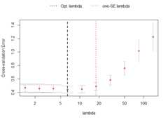
Further investigation into the model can be done by using thefunctionlagmatrix, which returns the lagmatrix of theestimated autoregressive coefficients. If entry(i, j) = x, this means that the sparseestimator indicates the effect of time seriesj on time seriesi to last forx periods. Setting thereturnplot argument toTRUE will return aheatmap for better visual inspection.
LhatL1<-lagmatrix(fit=VAR.L1,returnplot=TRUE)
The lag matrix is typically sparse as it contains some empty (i.e.,zero) cells. However, VAR models estimated with a standard L1-penaltyare typically not easily interpretable as they select many high lagorder coefficients (i.e., large values in the lagmatrix).
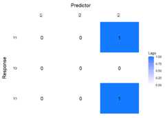
To circumvent this problem, we advise using a lag-basedhierarchically sparse estimation procedure, which boils down to usingthe default option HLag for theVARpen argument. Thisestimation procedure encourages low maximum lag orders, often results insparser lagmatrices, and hence more interpretable models.
Models can be estimated using the hierarchical penalization by usingthe default argument toVARpen, namelyHLag.Model selection can again be done by either settingselection="none" and obtaining a whole sequence of models,or by using any ofcv, bic, aic, hq.
VARHLag_none<-sparseVAR(Y=scale(Y.hlag),selection ="none")# HLag is the default VARpen optionVARHLag_cv<-sparseVAR(Y=scale(Y.hlag),selection ="cv")VARHLag_bic<-sparseVAR(Y=scale(Y.hlag),selection ="bic")# This will also give a table for IC comparison showing the selected lambda for each IC#>#>#> #### Selected the following lambda #####>#> AIC BIC HQ#> 10.74023 10.74023 10.74023#>#>#> #### Details #####>#> lambda AIC BIC HQ#> 1 138.7154 -0.9793 -0.9793 -0.9793#> 2 83.1577 -1.7792 -1.6473 -1.7258#> 3 49.8517 -3.0055 -2.7746 -2.912#> 4 29.8853 -4.1453 -3.8155 -4.0118#> 5 17.9158 -4.826 -4.4631 -4.6791#> 6 10.7402 ==> -5.0769 ==> -4.6151 ==> -4.89#> 7 6.4386 -5.0698 -4.3277 -4.7695#> 8 3.8598 -4.6703 -3.0377 -4.0096#> 9 2.3139 -2.7531 2.5737 -0.5974#> 10 1.3872 -1.5512 6.5956 1.7457Depending on which selection procedure was used, various diagnosticscan be produced. Former and foremost, all selection procedures supportthefitted andresiduals functions to obtainthe fitted and residual values respectively. Both functions return a 3Darray if the model usedselection="none" corresponding tothe fitted/residual values for each model in the penalizationsequence.
res_VARHLag_none<-residuals(VARHLag_none)# This is a 3D arraydim(res_VARHLag_none)#> [1] 179 5 10When an actual selection method was used(cv, bic, aic, hq), then other diagnostic functions exist.Forcv,plot_cv could be used again, just asshown above. For all, thediagnostics_plot function can beused to obtain a plot of fitted and residual values.
p_bic<-diagnostics_plot(VARHLag_bic,variable ="Y3")# variable argument can be numeric or characterp_cv<-diagnostics_plot(VARHLag_cv,variable ="Y3")# variable argument can be numeric or characterplot(p_bic)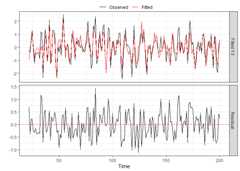
plot(p_cv)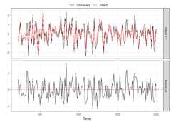
Often practitioners are interested in incorporating the impact ofunmodeled exogenous variables (X) into the VAR model. To do this, youcan use thesparseVARX function which has an argumentX where you can enter the data matrix of exogenous timeseries. For demonstration purposes, we will use thevarx.example data set that is part of bigtime.
data(varx.example)When applying thelagmatrix function to an estimatedsparse VARX model, the lag matrices of both the endogenous and exogenousautoregressive coefficients are returned.
sparseVARX supports the sameselectionarguments assparseVAR:none, cv, bic, aic, hq, and it is again recommended tostandardise the data.
VARXfit_cv<-sparseVARX(Y=scale(Y.varx),X=scale(X.varx),selection ="cv")LhatVARX<-lagmatrix(fit=VARXfit_cv,returnplot=TRUE)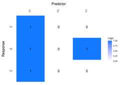
VARX models also supportplot_cv if estimated using CV.The returned plot shows the mean MSFE for each combination ofpenalizations in a heatmap. The x-axis show the penalizations for theexogenous variables, and the y-axis shows the penalizations for theendogenous variables. The big black dot in the plot below indicates theone-SE optimal choice, while the contours indicate the mean MSFE in theCV procedure. The red colour indicates a high MSFE, and light-yellow toyellow regions indicate low MSFEs.
plot_cv(VARXfit_cv)
Ifselection="none" a 3D array will be returned again.Although not mentioned previously, when settingselectiontonone, or any of the IC, one can also easily provide apenalization sequence, or even just ask for a single penalizationsetting. For example, below we intentionally choose a single, smallpenalization for the exogenous variables.
VARXfit_none<-sparseVARX(Y=scale(Y.varx),X=scale(X.varx),VARXlBseq =0.001,selection ="none")dim(VARXfit_none$Phihat)# This is a 3D array#> [1] 3 63 10# This is also 3D but third dimension is equal to ten# --> one penalization was chosen for B and 10 automatically for Phi# --> Cross product makes 10dim(VARXfit_none$Bhat)#> [1] 3 63 10Other functions such asresiduals,fitted,anddiagnostics_plot are also supported.
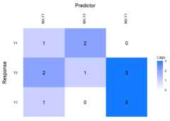
VARMA models generalise VAR models and often allow for moreparsimonious representations of the data generating process. To estimatea VARMA model to a multivariate time series data set, use the functionsparseVARMA, and choose a desired selection method. Thesparse VARMA estimation procedures consists of two stages: in the firststage a VAR model is estimated from which the residuals are retrieved.In the second stage these residuals are used as approximated error termsto estimate the VARMA model. As a default,sparseVARMA usesCV in the first stage andnone in the second stage.The first stage does not supportnone: A selectionneeds to be made.
Now lag matrices are obtained for the autoregressive (AR)coefficients and the moving average (MAs) coefficients.
data(varma.example)VARMAfit<-sparseVARMA(Y=scale(Y.varma),VARMAselection ="cv")# VARselection="cv" as default.LhatVARMA<-lagmatrix(fit=VARMAfit,returnplot=T)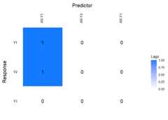
Other functions such asplot_cv,residuals,fitted anddiagnosticsplot are alsosupported.
To obtain forecasts from the estimated models, you can use thedirectforecast function for VAR, VARMA, and VARX, or therecursiveforecast function for VAR models. The defaultforecast horizon (argumenth) is set to one such thatone-step ahead forecasts are obtained, but you can specify your desiredforecast horizon.
Finally, we compare the forecast accuracy of the different models bycomparing their forecasts to the actual time series values of thevar.example data set that comes with bigtime. We willestimate all models using CV.
In this example, the VARMA model has the best forecast performance(i.e., lowest mean squared prediction error). This is somewhatsurprising given the data comes from a VAR model.
data(var.example)dim(Y.var)#> [1] 200 5Y<- Y.var[-nrow(Y.var), ]# leaving the last observation for comparisonYtest<- Y.var[nrow(Y.var), ]VARcv<-sparseVAR(Y =scale(Y),selection ="cv")VARMAcv<-sparseVARMA(Y =scale(Y),VARMAselection ="cv")Y<- Y.var[-nrow(Y.var),1:3]# considering first three variables as endogenousX<- Y.var[-nrow(Y.var),4:5]# and last two as exogenousVARXcv<-sparseVARX(Y =scale(Y),X =scale(X),selection ="cv")VARf<-directforecast(VARcv)# default is h=1VARXf<-directforecast(VARXcv)VARMAf<-directforecast(VARMAcv)# We can only compare forecasts for the first three variables# because VARX models only forecast endogenously modelled variablesmean((VARf[1:3]-Ytest[1:3])^2)#> [1] 0.6252039mean((VARXf[1:3]-Ytest[1:3])^2)#> [1] 0.6319843mean((VARMAf[1:3]-Ytest[1:3])^2)# lowest=best#> [1] 0.4571325Note that we could easily obtain longer horizon forecasts for the VARmodel by using therecursiveforecast function. It isrecommended to callis.stable first though, to checkwhether the obtained VAR model is stable.
is.stable(VARcv)#> [1] TRUErec_fcst<-recursiveforecast(VARcv,h =10)plot(rec_fcst,series ="Y2",last_n =50)# Plotting of a recursive forecast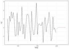
The functionssparseVAR,sparseVARX,sparseVARMA can also be used for the univariate settingwhere the response time seriesY is univariate. Below weillustrate the usefulness of the sparse estimation procedure asautomatic lag selection procedures.
We start by generating a time series of lengthn = 50 from astationary AR model and by plotting it. ThesparseVARfunction can also be used in the univariate case as it allows theargumentY to be a vector.
Thelagmatrix function gives the selected autoregressiveorder of the sparse AR model. The true order is one.
periods<-50k<-1p<-1sim_data<-simVAR(periods, k, p,sparsity_pattern ="none",max_abs_eigval =0.5,seed =123456)summary(sim_data)#> #### General Information #####>#> Seed 123456#> Time series length 50#> Burnin 50#> Variables Simulated 1#> Number of Lags 1#> Coefficients were randomly created? TRUE#> Maximum Eigenvalue of Companion Matrix 0.5#> Sparsity Pattern none#>#>#> #### Sparsity Options #####>#> NULL#>#>#> #### Coefficient Matrix #####>#> [,1]#> [1,] 0.4998982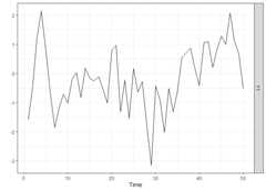
y<-scale(sim_data$Y)ARfit<-sparseVAR(Y=y,selection ="cv")lagmatrix(ARfit)#> $LPhi#> [,1]#> [1,] 1Note that all diagnostics functions discussed for the VAR, VARMA,VARX cases also work for univariate cases; so do the forecastingfunctions.
We start by generating a time series of lengthn = 50 from astationary ARX model and by plotting it. ThesparseVARXfunction can also be used in the univariate case as it allows theargumentsY andX to be vectors. Thelagmatrix function gives the selected endogenous (underLPhi) and exogenous autoregressive (underLB)orders of the sparse ARX model. The true orders are one.
periods<-50k<-1p<-1burnin<-100Xsim<-simVAR(periods+burnin+1, k, p,max_abs_eigval =0.8,seed =123)edist<-lag(Xsim$Y)[-1, ]+rnorm(periods+ burnin,sd =0.1)Ysim<-simVAR(periods, k , p,max_abs_eigval =0.5,seed =789,e_dist =t(edist),burnin = burnin)plot(Ysim)
x<-scale(Xsim$Y[-(1:(burnin+1))])y<-scale(Ysim$Y)ARXfit<-sparseVARX(Y=y,X=x,selection ="cv")lagmatrix(fit=ARXfit)#> $LPhi#> [,1]#> [1,] 1#>#> $LB#> [,1]#> [1,] 2We start by generating a time series of lengthn = 50 from astationary ARMA model and by plotting it. ThesparseVARMAfunction can also be used in the univariate case as it allows theargumentY to be a vector. Thelagmatrixfunction gives the selected autoregressive (underLPhi) andmoving average (underLTheta) orders of the sparse ARMAmodel. The true orders are one.
periods<-50k<-1p.u<-1p.y<-1burnin<-100u<-rnorm(periods+1+ burnin,sd =0.1)u<-embed(u,dimension = p.u+1)u<- u*matrix(rep(c(1,0.2),nrow(u)),nrow =nrow(u),byrow =TRUE)# Second column is lagged, first is current erroredist<-rowSums(u)Ysim<-simVAR(periods, k, p,e_dist =t(edist),max_abs_eigval =0.5,seed =789,burnin = burnin)summary(Ysim)#> #### General Information #####>#> Seed 789#> Time series length 50#> Burnin 100#> Variables Simulated 1#> Number of Lags 1#> Coefficients were randomly created? TRUE#> Maximum Eigenvalue of Companion Matrix 0.5#> Sparsity Pattern none#>#>#> #### Sparsity Options #####>#> NULL#>#>#> #### Coefficient Matrix #####>#> [,1]#> [1,] 0.4989384
ARMAfit<-sparseVARMA(Y=y,VARMAselection ="cv")lagmatrix(fit=ARMAfit)#> $LPhi#> [,1]#> [1,] 3#>#> $LTheta#> [,1]#> [1,] 0For a non-technical introduction to VAR models see this interactivenotebookand for an interactive notebook demonstrating the use of bigtime forhigh-dimensional VARs, see thisnotebook.Note: Loading these notebooks sometimes can take quite some time.Please be patient or try another time.
Nicholson William B., Wilms Ines, Bien Jacob and Matteson DavidS. (2020), “High-dimensional forecasting via interpretable vectorautoregression”, Journal of Machine Learning Research, 21(166),1-52.
Wilms Ines, Basu Sumanta, Bien Jacob and Matteson David S.(2021), “Sparse Identification and Estimation of Large-Scale VectorAutoRegressive Moving Averages”, Journal of the American StatisticalAssociation, doi: 10.1080/01621459.2021.1942013.
Wilms Ines, Basu Sumanta, Bien Jacob and Matteson David S.(2017), “Interpretable Vector AutoRegressions with Exogenous TimeSeries”, NIPS 2017 Symposium on Interpretable Machine Learning,arXiv:1711.03623