Movatterモバイル変換

Variable LengthMarkov Chains with Covariates

mixvlmc implements variable length Markov chains (VLMC)and variable length Markov chains with covariates (COVLMC), as describedin:

• Bühlmann, P. andWyner, A. J. (1999), Variable length Markov chains. Ann. Statist. 27 (2)480-513
• Zanin Zambom, A., Kim,S. and Lopes Garcia, N. (2022), Variable length Markov chain withexogenous covariates. J. Time Ser. Anal., 43 (2) 312-328

mixvlmc includes functionalities similar to the onesavailable inVLMCandPST. The mainadvantages ofmixvlmc are the support of time varyingcovariates with COVLMC and the introduction of post-pruning of themodels that enables fast model selection via information criteria.

Installation

The package can be installed from CRAN with:

install.packages("mixvlmc")

The development version is available from GitHub:

# install.packages("devtools")devtools::install_github("fabrice-rossi/mixvlmc")

Usage

Variable length Markovchains

Variable length Markov chains (VLMC) are sparse high order Markovchains. They can be used to model time series (sequences) with discretevalues (states) with a mix of small order dependencies for certainstates and higher order dependencies for other states. For instance,with a binary time series, the probability of observing 1 at time\(t\) could be constant whatever the olderpast states if the last one (at time\(t-1\)) was 1, but could depend on states attime\(t-3\) and\(t-2\) if the state was 0 at time\(t-1\). A collection of past states thatdetermines completely the transition probabilities is acontextof the VLMC. Readvignette("context-trees") for detailsabout contexts and context tree, and seevignette("variable-length-markov-chains") for a moredetailed introduction to VLMC.

VLMC with covariates (COVLMC) are extension of VLMC in whichtransition probabilities (probabilities of the next state given thepast) can be influenced by the past values of some covariates (inaddition to the past values of the time series itself). Each context isassociated to a logistic model that maps the (past values of the)covariates to transition probabilities.

Fitting a VLMC

The package is loaded in a standard way.

library(mixvlmc)library(ggplot2)

The main function of VLMC isvlmc() which can be calledon a time series represented by a numerical vector or a factor, forinstance.

set.seed(0)x<-sample(c(0L, 1L),200,replace =TRUE)model<-vlmc(x)model#> VLMC context tree on 0, 1#>  cutoff: 1.921 (quantile: 0.05)#>  Number of contexts: 11#>  Maximum context length: 6

The default parameters ofvlmc() will tend to produceoverly complex VLMC in order to avoid missing potential structure in thetime series. In the example above, we expect the optimal VLMC to be aconstant distribution as the sample is independent and uniformlydistributed (it has no temporal structure). The default parameters givehere an overly complex model, as illustrated by its text basedrepresentation

draw(model)#> * (0.505, 0.495)#> '-- 1 (0.4848, 0.5152)#>     +-- 0 (0.5319, 0.4681)#>     |   '-- 1 (0.5, 0.5)#>     |       '-- 0 (0.4444, 0.5556)#>     |           '-- 0 (0.4286, 0.5714)#>     |               +-- 0 (1, 0)#>     |               '-- 1 (0, 1)#>     '-- 1 (0.4314, 0.5686)#>         '-- 0 (0.2727, 0.7273)#>             '-- 0 (0.3846, 0.6154)#>                 '-- 0 (0.5, 0.5)#>                     +-- 0 (0, 1)#>                     '-- 1 (1, 0)

The representation uses simple ASCII art to display the contexts ofthe VLMC organized into a tree (seevignette("context-trees") for a more detailedintroduction):

• the root* corresponds to an empty context;
• one can read contexts by following branches (represented by 2 dashes--) down to their ends (the leaves): for instance\((0, 0, 0, 1, 0, 1)\) is one of the contextsof the tree.

Here the context\((0, 0, 0, 1, 0,1)\) is associated to the transition probabilities\((1, 0)\). This means that when one observesthis context in the time series, it isalways followed by a 0.Notice that contexts are extends to the left when we go down in the treeas deep nodes corresponds to older values. Some papers prefer to writecontexts from the most recent value to the oldest one. With thisconvention, the “reverse” context\((1, 0, 1,0, 0, 0)\) corresponds to the sub time series\((0, 0, 0, 1, 0, 1)\). Unless otherwisespecified, we write contexts in the temporal order.

BIC based model selection

The VLMC above is obviously overfitting to the time series, asillustrated by the 0/1 transition probabilities. A classical way toselect a good model is to minimize theBIC.Inmixvlmc this can be done easily using using‘tune_vlmc()’ which fits first a complex VLMC and thenprunesit (using a combination ofcutoff() andprune()), as follows (seevignette("variable-length-markov-chains") for details):

best_model_tune<-tune_vlmc(x)best_model<-as_vlmc(best_model_tune)draw(best_model)#> * (0.505, 0.495)

As expected, we end up with a constant model.

In time series with actual temporal patterns, the optimal model willbe more complex. As a very basic illustrative example, let us considerthesunspot.year time series and turn it into a binary one,with high activity associated to a number of sun spots larger than themedian number.

sun_activity<-as.factor(ifelse(sunspot.year>=median(sunspot.year),"high","low"))

We adjust automatically an optimal VLMC as follows:

sun_model_tune<-tune_vlmc(sun_activity)sun_model_tune#> VLMC context tree on high, low#>  cutoff: 2.306 (quantile: 0.03175)#>  Number of contexts: 9#>  Maximum context length: 5#>  Selected by BIC (236.262) with likelihood function "truncated" (-98.83247)

The results of the pruning process can be representedgraphically:

print(autoplot(sun_model_tune)+geom_point())

The plot shows that simpler models are too simple as the BICincreases when pruning becomes strong enough. The best model remainsrather complex (as expected based on the periodicity of the Solarcycle):

best_sun_model<-as_vlmc(sun_model_tune)draw(best_sun_model)#> * (0.5052, 0.4948)#> +-- high (0.8207, 0.1793)#> |   +-- high (0.7899, 0.2101)#> |   |   +-- high (0.7447, 0.2553)#> |   |   |   +-- high (0.6571, 0.3429)#> |   |   |   |   '-- low (0.9167, 0.08333)#> |   |   |   '-- low (1, 0)#> |   |   '-- low (0.96, 0.04)#> |   '-- low (0.9615, 0.03846)#> '-- low (0.1888, 0.8112)#>     +-- high (0, 1)#>     '-- low (0.2328, 0.7672)#>         +-- high (0, 1)#>         '-- low (0.3034, 0.6966)#>             '-- high (0.07692, 0.9231)

Fitting a VLMC withcovariates

To illustrate the use of covariates, we use the power consumptiondata set included in the package (seevignette("covlmc")for details). We consider a week of electricity usage as follows:

pc_week_5<- powerconsumption[powerconsumption$week==5, ]elec<- pc_week_5$active_powerggplot(pc_week_5,aes(x = date_time,y = active_power))+geom_line()+xlab("Date")+ylab("Activer power (kW)")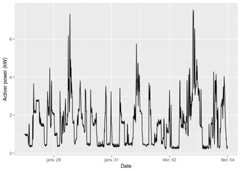

The time series displays some typical patterns of electricityusage:

• low active power at night (typically below 0.4 kW);
• standard use between 0.4 and 2 kW;
• peak use above 2 kW.

We build a discrete time series from those (somewhat arbitrary)thresholds:

elec_dts<-cut(elec,breaks =c(0,0.4,2,8),labels =c("low","typical","high"))

The best VLMC model is quite simple. It is almost a standard orderone Markov chain, up to the order 2 context used when the active poweristypical.

elec_vlmc_tune<-tune_vlmc(elec_dts)best_elec_vlmc<-as_vlmc(elec_vlmc_tune)draw(best_elec_vlmc)#> * (0.1667, 0.5496, 0.2837)#> +-- low (0.7665, 0.2335, 0)#> '-- typical (0.0704, 0.8466, 0.08303)#> |   '-- low (0.3846, 0.5385, 0.07692)#> '-- high (0.003497, 0.1573, 0.8392)

As pointed about above,low active power tend to correspondto night phase. We can include this information by introducing a daycovariate as follows:

elec_cov<-data.frame(day = (pc_week_5$hour>=7& pc_week_5$hour<=17))

A COVLMC is estimated using thecovlmc function:

elec_covlmc<-covlmc(elec_dts, elec_cov,min_size =2,alpha =0.5)draw(elec_covlmc,time_sep =" | ",model ="full",p_value =FALSE)#> *#> +-- low ([ (I)    | day_1TRUE#> |          -1.558 | 1.006     ])#> '-- typical#> |   +-- low ([ (I)    | day_1TRUE | day_2TRUE#> |   |          0.3567 | -27.81    | 27.81#> |   |          -1.253 | -14.39    | 13.69     ])#> |   '-- typical ([ (I)    | day_1TRUE#> |   |              2.666  | 0.566#> |   |              0.2683 | 0.2426    ])#> |   '-- high ([ (I)    | day_1TRUE#> |               2.015  | 16.18#> |               0.6931 | 16.61     ])#> '-- high ([ (I)   | day_1TRUE#>             17.41 | -14.23#>             19.38 | -14.88    ])

The model appears a bit complex. To get a more adapted model, we usea BIC based model selection as follows:

elec_covlmc_tune<-tune_covlmc(elec_dts, elec_cov)print(autoplot(elec_covlmc_tune))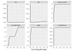

best_elec_covlmc<-as_covlmc(elec_covlmc_tune)draw(best_elec_covlmc,model ="full",time_sep =" | ",p_value =FALSE)#> *#> +-- low ([ (I)    | day_1TRUE#> |          -1.558 | 1.006     ])#> '-- typical#> |   +-- low ([ (I)#> |   |          0.3365#> |   |          -1.609 ])#> |   '-- typical ([ (I)#> |   |              2.937#> |   |              0.3747 ])#> |   '-- high ([ (I)#> |               2.773#> |               1.705 ])#> '-- high ([ (I)#>             3.807#>             5.481 ])

As in the VLMC case, the optimal model remains rather simple:

• thehigh context do not use the covariate and is equivalentto the vlmc context;
• thelow context is more interesting: it does not switch toahigh context (hence the single row of parameters) but usesthe covariate. As expected, the probability of switching fromlow totypical is larger during the day;
• thetypical context is described in a more complex way thatin the case of the vlmc as the transition probabilities depend on theprevious state.

Sampling

VLMC models can also be used to sample new time series as in the VMLCbootstrap proposed by Bühlmann and Wyner. For instance, we can estimatethe longest time period spent in thehigh active power regime.In this “predictive” setting, theAICmay be more adapted to select the best model. Notice that somequantities can be computed directly from the model in the VLMC case,using classical results on Markov Chains. Seevignette("sampling") for details on sampling.

We first select two models based on the AIC.

best_elec_vlmc_aic<-as_vlmc(tune_vlmc(elec_dts,criterion ="AIC"))best_elec_covlmc_aic<-as_covlmc(tune_covlmc(elec_dts, elec_cov,criterion ="AIC"))

The we sample 100 new time series for each model, using thesimulate() function as follows:

set.seed(0)vlmc_simul<-vector(mode ="list",100)for (kinseq_along(vlmc_simul)) {  vlmc_simul[[k]]<-simulate(best_elec_vlmc_aic,nsim =length(elec_dts),init = elec_dts[1:2])}

set.seed(0)covlmc_simul<-vector(mode ="list",100)for (kinseq_along(covlmc_simul)) {  covlmc_simul[[k]]<-simulate(best_elec_covlmc_aic,nsim =length(elec_dts),covariate = elec_cov,init = elec_dts[1:2])}

Then statistics can be computed on those time series. For instance,we look for the longest time period spent in thehigh activepower regime.

longuest_high<-function(x) {  high_length<-rle(x=="high")10*max(high_length$lengths[high_length$values])}lh_vlmc<-sapply(vlmc_simul, longuest_high)lh_covlmc<-sapply(covlmc_simul, longuest_high)

The average longest time spent inhigh consecutively is

• for the VLMC: 243.6 minutes with a standard error of 6.7337834;
• for the VLMC with covariate: 286 minutes with a standard error of8.9386235;
• 410 minutes for the observed time series.

The following figure shows the distributions of the times obtained byboth models as well as the observed value. The VLMC model with covariateis able to generate longer sequences in thehigh active powerstate than the bare VLMC model as the consequence of the sensitivity tothe day/night schedule.

lh<-data.frame(time =c(lh_vlmc, lh_covlmc),model =c(rep("VLMC",length(lh_vlmc)),rep("COVLMC",length(lh_covlmc))))ggplot(lh,aes(x = time,color = model))+geom_density()+geom_rug(alpha =0.5)+geom_vline(xintercept =longuest_high(elec_dts),color =3)

The VLMC with covariate can be used to investigate the effects ofchanges in those covariates. For instance, if the day time is longer, weexpecthigh power usage to be less frequent. For instance, wesimulate one week with a day time from 6:00 to 20:00 as follows.

elec_cov_long_days<-data.frame(day = (pc_week_5$hour>=6& pc_week_5$hour<=20))set.seed(0)covlmc_simul_ld<-vector(mode ="list",100)for (kinseq_along(covlmc_simul_ld)) {  covlmc_simul_ld[[k]]<-simulate(best_elec_covlmc_aic,nsim =length(elec_dts),covariate = elec_cov_long_days,init = elec_dts[1:2])}

As expected the distribution of the longest time spend consecutivelyinhigh power usage is shifted to lower values when the daylength is increased.

lh_covlmc_ld<-sapply(covlmc_simul_ld, longuest_high)day_time_effect<-data.frame(time =c(lh_covlmc, lh_covlmc_ld),`day length`=c(rep("Short days",length(lh_covlmc)),rep("Long days",length(lh_covlmc_ld))),check.names =FALSE)ggplot(day_time_effect,aes(x = time,color =`day length`))+geom_density()+geom_rug(alpha =0.5)