
Themargins andprediction packagesare a combined effort to port the functionality of Stata’s (closedsource)marginscommand to (open source) R. These tools provide ways of obtaining commonquantities of interest from regression-type models.margins provides “marginal effects” summaries of modelsandprediction provides unit-specific and sampleaverage predictions from models. Marginal effects are partialderivatives of the regression equation with respect to each variable inthe model for each unit in the data; average marginal effects are simplythe mean of these unit-specific partial derivatives over some sample. Inordinary least squares regression with no interactions or higher-orderterm, the estimated slope coefficients are marginal effects. In othercases and for generalized linear models, the coefficients are notmarginal effects at least not on the scale of the response variable.margins therefore provides ways of calculating themarginal effects of variables to make these models moreinterpretable.
The major functionality of Stata’smargins command -namely the estimation of marginal (or partial) effects - is providedhere through a single function,margins(). This is an S3generic method for calculating the marginal effects of covariatesincluded in model objects (like those of classes “lm” and “glm”). Usersinterested in generating predicted (fitted) values, such as the“predictive margins” generated by Stata’smargins command,should consider usingprediction() from the siblingproject,prediction.
With the introduction of Stata’smargins command, it hasbecome incredibly simple to estimate average marginal effects (i.e.,“average partial effects”) and marginal effects at representative cases.Indeed, in just a few lines of Stata code, regression results for almostany kind model can be transformed into meaningful quantities of interestand related plots:
. import delimited mtcars.csv. quietly reg mpg c.cyl##c.hp wt. margins, dydx(*)------------------------------------------------------------------------------ | Delta-method | dy/dx Std. Err. t P>|t| [95% Conf. Interval]-------------+---------------------------------------------------------------- cyl | .0381376 .5998897 0.06 0.950 -1.192735 1.26901 hp | -.0463187 .014516 -3.19 0.004 -.076103 -.0165343 wt | -3.119815 .661322 -4.72 0.000 -4.476736 -1.762894------------------------------------------------------------------------------. marginsplot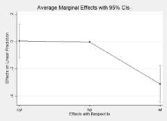
Stata’smargins command is incredibly robust. It workswith nearly any kind of statistical model and estimation procedure,including OLS, generalized linear models, panel regression models, andso forth. It also represents a significant improvement over Stata’sprevious marginal effects command -mfx - which was subjectto various well-known bugs. While other Stata modules have providedfunctionality for deriving quantities of interest from regressionestimates (e.g.,Clarify), none has done sowith the simplicity and genearlity ofmargins.
By comparison, R has no robust functionality in the base tools fordrawing out marginal effects from model estimates (though the S3predict() methods implement some of the functionality forcomputing fitted/predicted values). The closest approximation ismodmarg, whichdoes one-variable-at-a-time estimation of marginal effects is quiterobust. Other than this relatively new package on the scene, no packagesimplement appropriate marginal effect estimates. Notably, severalpackages provide estimates of marginal effects for different types ofmodels. Among these arecar,alr3,mfx,erer, among others.Unfortunately, none of these packages implement marginal effectscorrectly (i.e., correctly account for interrelated variables such asinteraction terms (e.g.,a:b) or power terms (e.g.,I(a^2)) and the packages all implement quite differentinterfaces for different types of models.interflex,interplot, andplotMElmprovide functionality simply for plotting quantities of interest frommultiplicative interaction terms in models but do not appear to supportgeneral marginal effects displays (in either tabular or graphical form),whilevisregprovides a more general plotting function but no tabular output.interactionTestprovides some additional useful functionality for controlling the falsediscovery rate when making such plots and interpretations, but is againnot a general tool for marginal effect estimation.
Given the challenges of interpreting the contribution of a givenregressor in any model that includes quadratic terms, multiplicativeinteractions, a non-linear transformation, or other complexities, thereis a clear need for a simple, consistent way to estimate marginaleffects for popular statistical models. This package aims to correctlycalculate marginal effects that include complex terms and provide auniform interface for doing those calculations. Thus, the packageimplements a single S3 generic method (margins()) that canbe easily generalized for any type of model implemented in R.
Some technical details of the package are worth briefly noting. Theestimation of marginal effects relies on numerical approximations ofderivatives produced usingpredict() (actually, a wrapperaroundpredict() calledprediction() that istype-safe). Variance estimation, by default is provided using the deltamethod a numerical approximation oftheJacobian matrix. While symbolic differentiation of some models(e.g., basic linear models) is possible usingD() andderiv(), R’s modelling language (the “formula” class) issufficiently general to enable the construction of model formulae thatcontain terms that fall outside of R’s symbolic differentiation ruletable (e.g.,y ~ factor(x) ory ~ I(FUN(x))for any arbitraryFUN()). By relying on numericdifferentiation,margins() supportsany model thatcan be expressed in R formula syntax. Even Stata’smarginscommand is limited in its ability to handle variable transformations(e.g., includingx andlog(x) as predictors)and quadratic terms (e.g.,x^3); these scenarios are easilyexpressed in an R formula and easily handled, correctly, bymargins().
Replicating Stata’s results is incredibly simple using just themargins() method to obtain average marginal effects:
library("margins")mod1<-lm(mpg~ cyl* hp+ wt,data = mtcars)(marg1<-margins(mod1))## Average marginal effects## lm(formula = mpg ~ cyl * hp + wt, data = mtcars)## cyl hp wt## 0.03814 -0.04632 -3.12summary(marg1)## factor AME SE z p lower upper## cyl 0.0381 0.5999 0.0636 0.9493 -1.1376 1.2139## hp -0.0463 0.0145 -3.1909 0.0014 -0.0748 -0.0179## wt -3.1198 0.6613 -4.7175 0.0000 -4.4160 -1.8236With the exception of differences in rounding, the above resultsmatch identically what Stata’smargins command produces. Aslightly more concise expression relies on the syntactic sugar providedbymargins_summary():
margins_summary(mod1)## factor AME SE z p lower upper## cyl 0.0381 0.5999 0.0636 0.9493 -1.1376 1.2139## hp -0.0463 0.0145 -3.1909 0.0014 -0.0748 -0.0179## wt -3.1198 0.6613 -4.7175 0.0000 -4.4160 -1.8236If you are only interested in obtaining the marginal effects (withoutcorresponding variances or the overhead of creating a “margins” object),you can callmarginal_effects(x) directly. Furthermore, thedydx() function enables the calculation of the marginaleffect of a single named variable:
# all marginal effects, as a data.framehead(marginal_effects(mod1))## dydx_cyl dydx_hp dydx_wt## 1 -0.6572244 -0.04987248 -3.119815## 2 -0.6572244 -0.04987248 -3.119815## 3 -0.9794364 -0.08777977 -3.119815## 4 -0.6572244 -0.04987248 -3.119815## 5 0.5747624 -0.01196519 -3.119815## 6 -0.7519926 -0.04987248 -3.119815# subset of all marginal effects, as a data.framehead(marginal_effects(mod1,variables =c("cyl","hp")))## dydx_cyl dydx_hp## 1 -0.6572244 -0.04987248## 2 -0.6572244 -0.04987248## 3 -0.9794364 -0.08777977## 4 -0.6572244 -0.04987248## 5 0.5747624 -0.01196519## 6 -0.7519926 -0.04987248# marginal effect of one variablehead(dydx(mtcars, mod1,"cyl"))## dydx_cyl## 1 -0.6572244## 2 -0.6572244## 3 -0.9794364## 4 -0.6572244## 5 0.5747624## 6 -0.7519926These functions may be useful for plotting, getting a quickimpression of the results, or for using unit-specific marginal effectsin further analyses.
at) and Subgroup AnalysesThe package also implement’s one of the best features ofmargins, which is theat specification thatallows for the estimation of average marginal effects for counterfactualdatasets in which particular variables are held at fixed values:
# webuse margexlibrary("webuse")webuse::webuse("margex")# logistic outcome treatment##group age c.age#c.age treatment#c.agemod2<-glm(outcome~ treatment* group+ age+I(age^2)* treatment,data = margex,family = binomial)# margins, dydx(*)summary(margins(mod2))## factor AME SE z p lower upper## age 0.0096 0.0008 12.3763 0.0000 0.0081 0.0112## group -0.0479 0.0129 -3.7044 0.0002 -0.0733 -0.0226## treatment 0.0432 0.0147 2.9321 0.0034 0.0143 0.0720# margins, dydx(treatment) at(age=(20(10)60))summary(margins(mod2,at =list(age =c(20,30,40,50,60)),variables ="treatment"))## factor age AME SE z p lower upper## treatment 20.0000 -0.0009 0.0043 -0.2061 0.8367 -0.0093 0.0075## treatment 30.0000 0.0034 0.0107 0.3200 0.7490 -0.0176 0.0245## treatment 40.0000 0.0301 0.0170 1.7736 0.0761 -0.0032 0.0634## treatment 50.0000 0.0990 0.0217 4.5666 0.0000 0.0565 0.1415## treatment 60.0000 0.1896 0.0384 4.9339 0.0000 0.1143 0.2649This functionality removes the need to modify data before performingsuch calculations, which can be quite unwieldy when many specificationsare desired.
If one desiressubgroup effects, simply pass a subset ofdata to thedata argument:
# effects for mensummary(margins(mod2,data =subset(margex, sex==0)))## factor AME SE z p lower upper## age 0.0043 0.0007 5.7723 0.0000 0.0028 0.0057## group -0.0753 0.0105 -7.1745 0.0000 -0.0959 -0.0547## treatment 0.0381 0.0070 5.4618 0.0000 0.0244 0.0517# effects for wommensummary(margins(mod2,data =subset(margex, sex==1)))## factor AME SE z p lower upper## age 0.0150 0.0013 11.5578 0.0000 0.0125 0.0176## group -0.0206 0.0236 -0.8742 0.3820 -0.0669 0.0256## treatment 0.0482 0.0231 2.0910 0.0365 0.0030 0.0934The package implements several useful additional features forsummarizing model objects, including:
plot() method for the new “margins” class that portsStata’smarginsplot command.cplot() to provide the commonlyneeded visual summaries of predictions or average marginal effectsconditional on a covariate.persp() method for “lm”, “glm”, and “loess” objectsto provide three-dimensional representations of response surfaces ormarginal effects over two covariates.image() method for the same that produces flat,two-dimensional heatmap-style representations ofpersp()-type plots.Using theplot() method yields an aesthetically similarresult to Stata’smarginsplot:
library("webuse")webuse::webuse("nhanes2")mod3<-glm(highbp~ sex* agegrp* bmi,data = nhanes2,family = binomial)summary(marg3<-margins(mod3))## factor AME SE z p lower upper## agegrp 0.0846 0.0021 39.4392 0.0000 0.0804 0.0888## bmi 0.0261 0.0009 28.4995 0.0000 0.0243 0.0279## sex -0.0911 0.0085 -10.7063 0.0000 -0.1077 -0.0744plot(marg3)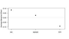
In addition to the estimation procedures andplot()generic,margins offers several plotting methods formodel objects. First, there is a new genericcplot() thatdisplays predictions or marginal effects (from an “lm” or “glm” model)of a variable conditional across values of third variable (or itself).For example, here is a graph of predicted probabilities from a logitmodel:
mod4<-glm(am~ wt*drat,data = mtcars,family = binomial)cplot(mod4,x ="wt",se.type ="shade")
And fitted values with a factor independent variable:
cplot(lm(Sepal.Length~ Species,data = iris))
and a graph of the effect ofdrat across levels ofwt:
cplot(mod4,x ="wt",dx ="drat",what ="effect",se.type ="shade")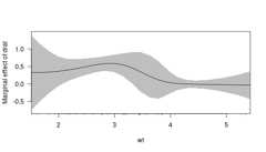
cplot() also returns a data frame of values, so that itcan be used just for calculating quantities of interest before plottingthem with another graphics package, such asggplot2:
library("ggplot2")dat<-cplot(mod4,x ="wt",dx ="drat",what ="effect",draw =FALSE)head(dat)## xvals yvals upper lower factor## 1.5130 0.3250 1.3927 -0.7426 drat## 1.6760 0.3262 1.1318 -0.4795 drat## 1.8389 0.3384 0.9214 -0.2447 drat## 2.0019 0.3623 0.7777 -0.0531 drat## 2.1648 0.3978 0.7110 0.0846 drat## 2.3278 0.4432 0.7074 0.1789 dratggplot(dat,aes(x = xvals))+geom_ribbon(aes(ymin = lower,ymax = upper),fill ="gray70")+geom_line(aes(y = yvals))+xlab("Vehicle Weight (1000s of lbs)")+ylab("Average Marginal Effect of Rear Axle Ratio")+ggtitle("Predicting Automatic/Manual Transmission from Vehicle Characteristics")+theme_bw()
Second, the package implements methods for “lm” and “glm” classobjects for thepersp() generic plotting function. Thisenables three-dimensional representations of predicted outcomes:
persp(mod1,xvar ="cyl",yvar ="hp")
and marginal effects:
persp(mod1,xvar ="cyl",yvar ="hp",what ="effect",nx =10)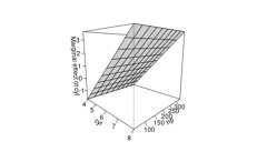
And if three-dimensional plots aren’t your thing, there are alsoanalogous methods for theimage() generic, to produceheatmap-style representations:
image(mod1,xvar ="cyl",yvar ="hp",main ="Predicted Fuel Efficiency,\nby Cylinders and Horsepower")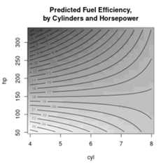
The numerous package vignettes and help files contain extensivedocumentation and examples of all package functionality.
While there is still work to be done to improve performance,margins is reasonably speedy:
library("microbenchmark")microbenchmark(marginal_effects(mod1))## Unit: milliseconds## expr min lq mean median uq max neval## marginal_effects(mod1) 2.256082 2.274596 2.414173 2.283578 2.304247 10.75537 100microbenchmark(margins(mod1))## Unit: milliseconds## expr min lq mean median uq max neval## margins(mod1) 16.62163 16.8786 17.80402 17.20959 17.67329 24.95876 100The most computationally expensive part ofmargins() isvariance estimation. If you don’t need variances, usemarginal_effects() directly or specifymargins(..., vce = "none").


The development version of this package can be installed directlyfrom GitHub usingremotes:
if (!require("remotes")) {install.packages("remotes")library("remotes")}install_github("leeper/prediction")install_github("leeper/margins")# building vignettes takes a moment, so for a quicker install set:install_github("leeper/margins",build_vignettes =FALSE)