Movatterモバイル変換

Contents

• Introduction
• Example: Arule ensemble for predicting ozone levels
• Tools for interpretation
  • Importance measures
  • Explaining individualpredictions
  • Partial dependenceplots
  • Assessing presence ofinteractions
  • Correlations betweenselected terms
• Tuning parameters of functionpre
• Dealing with missingvalues
• Go sparser withrelaxed lasso fits
• GeneralizedPrediction Ensembles: Combining MARS, rules and linear terms
• Credits
• References

Introduction

pre is anR packagefor deriving prediction rule ensembles for binary, multinomial,(multivariate) continuous, count and survival responses. Input variablesmay be numeric, ordinal and categorical. An extensive description of theimplementation and functionality is provided in Fokkema (2020). Thepackage largely implements the algorithm for deriving prediction ruleensembles as described in Friedman & Popescu (2008), with severaladjustments:

1. The package is completelyR based,allowing users better access to the results and more control over theparameters used for generating the prediction rule ensemble.
2. The unbiased tree induction algorithms of Hothorn, Hornik, &Zeileis (2006) is used for deriving prediction rules, by default.Alternatively, the (g)lmtree algorithm of Zeileis, Hothorn, & Hornik(2008) can be employed, or the classification and regression tree (CART)algorithm of Breiman, Friedman, Olshen, & Stone (1984).
3. The package supports a wider range of response variable types.
4. The initial ensemble may be generated as a bagged, boosted and/orrandom forest ensemble.
5. Hinge functions of predictor variables may be included asbaselearners, as in the multivariate adaptive regression splines (MARS)approach of Friedman (1991), using functiongpe().
6. Tools for explaining individual predictions are provided.

Note thatpre is under development, andmuch work still needs to be done. Below, an introduction the the packageis provided. Fokkema (2020) provides an extensive description of thefitting procedures implemented in functionpre() andexample analyses with more extensive explanations. An extensiveintroduction aimed at researchers in social sciences is provided inFokkema & Strobl (2020).

Example: Arule ensemble for predicting ozone levels

To get a first impression of how functionpre() works,we will predict Ozone levels using theairquality dataset.We fit a prediction rule ensemble using functionpre():

library("pre")airq<- airquality[complete.cases(airquality), ]set.seed(42)airq.ens<-pre(Ozone~ .,data = airq)

Note that it is necessary to set the random seed, to allow for laterreplication of results, because the fitting procedure depends on randomsampling of training observations.

We can print the resulting ensemble (alternatively, we could use theprint method):

airq.ens#>#> Final ensemble with cv error within 1se of minimum:#>#>   lambda =  3.543968#>   number of terms = 12#>   mean cv error (se) = 352.395 (99.13754)#>#>   cv error type : Mean-Squared Error#>#>          rule   coefficient                          description#>   (Intercept)   68.48270407                                    1#>       rule191  -10.97368180              Wind > 5.7 & Temp <= 87#>       rule173  -10.90385519              Wind > 5.7 & Temp <= 82#>        rule42   -8.79715538              Wind > 6.3 & Temp <= 84#>       rule204    7.16114781         Wind <= 10.3 & Solar.R > 148#>        rule10   -4.68646145              Temp <= 84 & Temp <= 77#>       rule192   -3.34460038  Wind > 5.7 & Temp <= 87 & Day <= 23#>        rule51   -2.27864287              Wind > 5.7 & Temp <= 84#>        rule93    2.18465676              Temp > 77 & Wind <= 8.6#>        rule74   -1.36479545              Wind > 6.9 & Temp <= 84#>        rule28   -1.15326093              Temp <= 84 & Wind > 7.4#>        rule25   -0.70818400              Wind > 6.3 & Temp <= 82#>       rule166   -0.04751152              Wind > 6.9 & Temp <= 82

The first few lines of the printed results provide the penaltyparameter value (λ) employed for selecting the final ensemble.By default, the ‘1-SE’ rule is used for selectingλ; thisdefault can be overridden by employing thepenalty.par.valargument of theprint method and other functions in thepackage. Note that the printed cross-validated error is calculated usingthe same data as was used for generating the rules and likely providesan overly optimistic estimate of future prediction error. To obtain amore realistic prediction error estimate, we will use functioncvpre() later on.

Next, the printed results provide the rules and linear terms selectedin the final ensemble, with their estimated coefficients. For rules, thedescription column provides the conditions. For linearterms (which were not selected in the current ensemble), the winsorizingpoints used to reduce the influence of outliers on the estimatedcoefficient would be printed in thedescription column. Thecoefficient column presents the estimated coefficient.These are regression coefficients, reflecting the expected increase inthe response for a unit increase in the predictor, keeping all otherpredictors constant. For rules, the coefficient thus reflects thedifference in the expected value of the response when the conditions ofthe rule are met, compared to when they are not.

Using theplot method, we can plot the rules in theensemble as simple decision trees. Here, we will request the nine mostimportant baselearners through specification of thentermsargument. Through thecex argument, we specify the size ofthe node and path labels:

plot(airq.ens,nterms =9,cex = .5)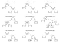

Using thecoef method, we can obtain the estimatedcoefficients for each of the baselearners (we only print the first sixterms here for space considerations):

coefs<-coef(airq.ens)coefs[1:6, ]#>            rule coefficient                  description#> 201 (Intercept)   68.482704                            1#> 167     rule191  -10.973682      Wind > 5.7 & Temp <= 87#> 150     rule173  -10.903855      Wind > 5.7 & Temp <= 82#> 39       rule42   -8.797155      Wind > 6.3 & Temp <= 84#> 179     rule204    7.161148 Wind <= 10.3 & Solar.R > 148#> 10       rule10   -4.686461      Temp <= 84 & Temp <= 77

We can generate predictions for new observations using thepredict method (only the first six predicted values areprinted here for space considerations):

predict(airq.ens,newdata = airq[1:6, ])#>        1        2        3        4        7        8#> 32.53896 24.22456 24.22456 24.22456 31.38570 24.22456

Using functioncvpre(), we can assess the expectedprediction error of the fitted PRE throughk-fold crossvalidation (k = 10, by default, which can be overridden throughspecification of thek argument):

set.seed(43)airq.cv<-cvpre(airq.ens)#> $MSE#>       MSE        se#> 369.92747  88.65343#>#> $MAE#>       MAE        se#> 13.666860  1.290329

The results provide the mean squared error (MSE) and mean absoluteerror (MAE) with their respective standard errors. These results aresaved for later use inaiq.cv$accuracy. The cross-validatedpredictions, which can be used to compute alternative estimates ofpredictive accuracy, are saved inairq.cv$cvpreds. Thefolds to which observations were assigned are saved inairq.cv$fold_indicators.

For tuning the parameters of functionpre() so as toobtain optimal predictive accuracy, users are advised to useR packagecaret. A tutorial is provided as avignette, accessible by typingvignette("tuning", package = "pre") inR or by going tohttps://cran.r-project.org/package=pre/vignettes/missingness.htmlin a browser and clicking on the corresponding link to the vignette.

Tools for interpretation

Packagepre provides several additionaltools for interpretation of the final ensemble. These may be especiallyhelpful for complex ensembles containing many rules and linearterms.

Importance measures

We can assess the relative importance of input variables as well asbaselearners using theimportance() function:

imps<-importance(airq.ens,round =4)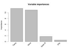

As we already observed in the printed ensemble, the plotted variableimportances indicate that Temperature and Wind are most stronglyassociated with Ozone levels. Solar.R and Day are also associated withOzone levels, but much less strongly. Variable Month is not plotted,which means it obtained an importance of zero, indicating that it is notassociated with Ozone levels. We already observed this in the printedensemble: Month did not appear in any of the selected terms. Thevariable and baselearner importances are saved for later use inimps$varimps andimps$baseimps,respectively.

Explaining individualpredictions

We can obtain explanations of the predictions for individualobservations using functionexplain():

par(mfrow =c(1,2))expl<-explain(airq.ens,newdata = airq[1:2, ],cex = .8)

The values of the rules and linear terms for each observation aresaved inexpl$predictors, their contributions inexpl$contribution and the predicted values inexpl$predicted.value.

Partial dependence plots

We can obtain partial dependence plots to assess the effect of singlepredictor variables on the outcome using thesingleplot()function:

singleplot(airq.ens,varname ="Temp")

We can obtain partial dependence plots to assess the effects of pairsof predictor variables on the outcome using thepairplot()function:

pairplot(airq.ens,varnames =c("Temp","Wind"))

Note that creating partial dependence plots is computationallyintensive and computation time will increase fast with increasingnumbers of observations and numbers of variables. Milborrow’s (2018)plotmo package provides more efficientfunctions for plotting partial dependence, which also supportpre models.

If the final ensemble does not contain many terms, inspectingindividual rules and linear terms through theprint methodmay be more informative than partial dependence plots. One of the mainadvantages of prediction rule ensembles is their interpretability: thepredictive model contains only simple functions of the predictorvariables (rules and linear terms), which are easy to grasp. Partialdependence plots are often much more useful for interpretation ofcomplex models, like random forests for example.

Assessing presence ofinteractions

We can assess the presence of interactions between the inputvariables using theinteract() andbsnullinteract() funtions. Functionbsnullinteract() computes null-interaction models (10, bydefault) based on bootstrap-sampled and permuted datasets. Functioninteract() computes interaction test statistics for eachpredictor variables appearing in the specified ensemble. Ifnull-interaction models are provided through thenullmodsargument, interaction test statistics will also be computed for thenull-interaction model, providing a reference null distribution.

Note that computing null interaction models and interaction teststatistics is computationally very intensive, so running the followingcode will take some time:

set.seed(44)nullmods<-bsnullinteract(airq.ens)int<-interact(airq.ens,nullmods = nullmods)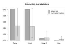

The plotted variable interaction strengths indicate that Temperatureand Wind may be involved in interactions, as their observed interactionstrengths (darker grey) exceed the upper limit of the 90% confidenceinterval (CI) of interaction stengths in the null interaction models(lighter grey bar represents the median, error bars represent the 90%CIs). The plot indicates that Solar.R and Day are not involved in anyinteractions. Note that computation of null interaction models iscomputationally intensive. A more reliable result can be obtained bycomputing a larger number of boostrapped null interaction datasets, bysetting thensamp argument of functionbsnullinteract() to a larger value (e.g., 100).

Correlations betweenselected terms

We can assess correlations between the baselearners appearing in theensemble using thecorplot() function:

corplot(airq.ens)

Tuning parameters

To obtain an optimal set of model-fitting parameters, packagecaret Kuhn (2008) provides a method"pre". For a manual on how to optimize the parameters offunctionpre usingcaret’strain function, see the vignette on tuning:

vignette("tuning",package ="pre")

or go tohttps://cran.r-project.org/package=pre/vignettes/tuning.htmlin a browser.

Dealing with missing values

Some suggestions on how to deal with missing values are provided inthe following vignette:

vignette("missingness",package ="pre")

or go tohttps://cran.r-project.org/package=pre/vignettes/missingness.htmlin a browser.

Go sparser with relaxedlasso fits

When sparsity (i.e., a final ensemble comprising only few terms) isof central importance, the so-called relaxed lasso can be employed. Itallows for retaining a pre-specified (low) number of terms, withadequate predictive accuracy. An introduction and tutorial is providedin the following vignette:

vignette("relaxed",package ="pre")

set.seed(42)airq.gpe<-gpe(Ozone~ .,data = airquality[complete.cases(airquality),],base_learners =list(gpe_trees(),gpe_linear(),gpe_earth()))airq.gpe#>#> Final ensemble with cv error within 1se of minimum:#>#>   lambda =  3.229132#>   number of terms = 11#>   mean cv error (se) = 359.2623 (110.8863)#>#>   cv error type : Mean-squared Error#>#>                                   description  coefficient#>                                   (Intercept)  65.52169488#>                                    Temp <= 77  -6.20973855#>                  Wind <= 10.3 & Solar.R > 148   5.46410966#>                       Wind > 5.7 & Temp <= 82  -8.06127415#>                       Wind > 5.7 & Temp <= 84  -7.16921733#>                       Wind > 5.7 & Temp <= 87  -8.04255471#>           Wind > 5.7 & Temp <= 87 & Day <= 23  -3.40525575#>                       Wind > 6.3 & Temp <= 82  -2.71925536#>                       Wind > 6.3 & Temp <= 84  -5.99085126#>                       Wind > 6.9 & Temp <= 82  -0.04406376#>                       Wind > 6.9 & Temp <= 84  -0.55827336#>   eTerm(Solar.R * h(9.7 - Wind), scale = 410)   9.91783320#>#>   'h' in the 'eTerm' indicates the hinge function