

This package implements z-curves - methods for estimating expecteddiscovery and replicability rates on bases of test-statistics ofpublished studies. The package provides functions for fitting thecensored EM version (Schimmack & Bartoš, 2023), the EM version(Bartoš & Schimmack, 2022) as well as the original density z-curve(Brunner & Schimmack, 2020). Furthermore, the package providessummarizing and plotting functions for the fitted z-curve objects. Seethe aforementioned articles for more information about z-curve, expecteddiscovery rate (EDR), expected replicability rate (ERR), maximum falsediscovery rate (FDR), as well as validation studies, andlimitations.
You can install the current version of zcurve from CRAN with:
install.packages("zcurve")or the development version fromGitHub with:
# install.packages("devtools")devtools::install_github("FBartos/zcurve")Z-curve can be used to estimate expected replicability rate (ERR),expected discovery rate (EDR), and maximum false discovery rate (SoricFDR) using z-scores from a set of significant findings. This is areproduction of an example in Bartoš and Schimmack (2022) where thez-curve is used to estimate ERR and EDR on a subset of studies used inreproducibility project (OSC, 2015). Only studies with non-ambiguousoriginal outcomes are used - excluding studies with “marginallysignificant” original findings, leading to 90 studies. Out of these 90studies, 35 were successfully replicated.
We included the recoded z-scores from the 90 OSC studies as a datasetin the package (‘OSC.z’). The expectation-maximization (EM) version ofthe z-curve is implemented as the default method and can be fitted (with1000 bootstraps) and summarized using ‘zcurve and ’summary’functions.
The first argument to the function call is a vector of z-scores.Alternatively, a vector of two-sided p-values can be also used, byspecifying “zcurve(p = p.values)”.
set.seed(666)library(zcurve)fit<-zcurve(OSC.z)summary(fit)#> Call:#> zcurve(z = OSC.z)#>#> model: EM via EM#>#> Estimate l.CI u.CI#> ERR 0.615 0.443 0.740#> EDR 0.388 0.070 0.699#>#> Model converged in 27 + 783 iterations#> Fitted using 73 z-values. 90 supplied, 85 significant (ODR = 0.94, 95% CI [0.87, 0.98]).#> Q = -60.61, 95% CI[-72.24, -46.24]More details from the fitted object can be extracted from the fittedobject. For more statistics, as expected number of conducted studies,the file drawer ratio or Sorić’s FDR specify ‘all = TRUE’ (see Schimmack& Bartoš, 2023) .
summary(fit,all =TRUE)#> Call:#> zcurve(z = OSC.z)#>#> model: EM via EM#>#> Estimate l.CI u.CI#> ERR 0.615 0.443 0.740#> EDR 0.388 0.070 0.699#> Soric FDR 0.083 0.023 0.705#> File Drawer R 1.574 0.430 13.387#> Expected N 219 122 1223#> Missing N 129 32 1133#>#> Model converged in 27 + 783 iterations#> Fitted using 73 z-values. 90 supplied, 85 significant (ODR = 0.94, 95% CI [0.87, 0.98]).#> Q = -60.61, 95% CI[-72.24, -46.24]For more information regarding the fitted model weights add ‘type =“parameters”’.
summary(fit,type ="parameters")#> Call:#> zcurve(z = OSC.z)#>#> model: EM via EM#>#> Mean Weight l.CI u.CI#> 1 0.000 0.056 0.000 0.445#> 2 1.000 0.005 0.000 0.374#> 3 2.000 0.734 0.002 0.999#> 4 3.000 0.205 0.000 0.640#> 5 4.000 0.000 0.000 0.000#> 6 5.000 0.000 0.000 0.000#> 7 6.000 0.000 0.000 0.000#>#> Model converged in 27 + 783 iterations#> Fitted using 73 z-values. 90 supplied, 85 significant (ODR = 0.94, 95% CI [0.87, 0.98]).#> Q = -60.61, 95% CI[-72.24, -46.24]The package also provides a convenient plotting method for thez-curve fits.
plot(fit)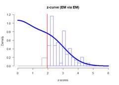
The default plot can be further modified by using classic R plottingarguments as ‘xlab’, ‘ylab’, ‘main’, ‘cex.axis’, ‘cex.lab’. Furthermore,an annotation with the main test statistics can be added to the plot byspecifying ‘annotation = TRUE’ and the pointwise confidence intervals ofthe plot by specifying “CI = TRUE”. For more options regarding theannotation see ’?plot.zcurve”.
plot(fit,CI =TRUE,annotation =TRUE,main ="OSC 2015")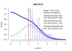
Other versions of the z-curves may be fitted by changing the methodargument in the ‘zcurve’ function. Set ‘method = “density”’ to fit thenew version of z-curve using density method (KD2). The original versionof the density method as implemented in Brunner and Schimmack (2020) canbe fitted by adding ‘list(model = “KD1”)’ to the ‘control’ argument of‘zcurve’.
(We omit bootstrapping to speed the fitting process in this case)
fit.KD2<-zcurve(OSC.z,method ="density",bootstrap =FALSE)fit.KD1<-zcurve(OSC.z,method ="density",control =list(model ="KD1"),bootstrap =FALSE)summary(fit.KD2)#> Call:#> zcurve(z = OSC.z, method = "density", bootstrap = FALSE)#>#> model: KD2 via density#>#> Estimate#> ERR 0.613#> EDR 0.506#>#> Model converged in 46 iterations#> Fitted using 73 z-values. 90 supplied, 85 significant (ODR = 0.94, 95% CI [0.87, 0.98]).#> RMSE = 0.11summary(fit.KD1)#> Call:#> zcurve(z = OSC.z, method = "density", bootstrap = FALSE, control = list(model = "KD1"))#>#> model: KD1 via density (version 1)#>#> Estimate#> ERR 0.637#>#> Model converged in 44 iterations#> Fitted using 73 z-values. 90 supplied, 85 significant (ODR = 0.94, 95% CI [0.87, 0.98]).#> MAE (*1e3) = 0.26The ‘control’ argument can be used to change the number of iterationsor reducing the convergence criterion in cases of non-convergence. Itcan be also used for constructing custom z-curves by changing thelocation of the mean components, their number or many other settings.However, it is important to bear in mind that those custom models needto be validated first on simulation studies prior to their usage. Formore information about the control settings see ‘?control_EM’,‘?control_density’, and ‘?control_density_v1’.
If you encounter any problems or bugs, please, contact me atf.bartos96[at]gmail.com or submit an issue athttps://github.com/FBartos/zcurve/issues. If you likethe package and use it in your work, please, cite it as:
citation(package ="zcurve")#> To cite the zcurve package in publications use:#>#> Bartoš F, Schimmack U (2020). "zcurve: An R Package for Fitting#> Z-curves." R package version 2.4.2,#> <https://CRAN.R-project.org/package=zcurve>.#>#> A BibTeX entry for LaTeX users is#>#> @Misc{,#> title = {zcurve: An R Package for Fitting Z-curves},#> author = {František Bartoš and Ulrich Schimmack},#> year = {2020},#> note = {R package version 2.4.2},#> url = {https://CRAN.R-project.org/package=zcurve},#> }Schimmack, U., & Bartoš, F. (2023). Estimating the falsediscovery risk of (randomized) clinical trials in medical journals basedon published p-values.PLoS ONE, 18(8), e0290084.https://doi.org/10.1371/journal.pone.0290084
Bartoš, F., & Schimmack, U. (2022). Z-curve 2.0: Estimatingreplication rates and discovery rates.Meta-Psychology, 6.https://doi.org/10.15626/MP.2021.2720
Brunner, J., & Schimmack, U. (2020). Estimating population meanpower under conditions of heterogeneity and selection for significance.Meta-Psychology, 4.https://doi.org/10.15626/MP.2018.874
Open Science Collaboration. (2015). Estimating the reproducibility ofpsychological science.Science, 349(6251), aac4716.https://doi.org/10.1126/science.aac4716