


The goal of theLMMsolver package is to fit(generalized) linear mixed models efficiently when the model structureis large or sparse. It provides tools for estimating variance componentsusing restricted maximum likelihood (REML) and is designed for modelsthat involve many random effects or smooth terms.
A key feature of the package is support for smoothing usingP-splines. LMMsolver uses a sparse formulation (Boer 2023), which makescomputations fast and memory efficient, especially for two-dimensionalsmoothing problems such as spatial surfaces or image-like data (Boer2023; Carollo et al. 2024).
This makesLMMsolver particularly useful forapplications involving spatial or temporal smoothing, large data sets,and models where standard mixed model tools become slow orimpractical.
install.packages("LMMsolver")remotes::install_github("Biometris/LMMsolver",ref ="develop",dependencies =TRUE)As an example of the functionality of the package we use theUSprecip data set in thespam package (Furrerand Sain 2010).
library(LMMsolver)library(ggplot2)## Get precipitation data from spamdata(USprecip,package ="spam")## Only use observed data.USprecip<-as.data.frame(USprecip)USprecip<- USprecip[USprecip$infill==1, ]head(USprecip[,c(1,2,4)],3)#> lon lat anomaly#> 6 -85.95 32.95 -0.84035#> 7 -85.87 32.98 -0.65922#> 9 -88.28 33.23 -0.28018A two-dimensional P-spline can be defined with thespl2D() function, with longitude and latitude ascovariates, and anomaly (standardized monthly total precipitation) asresponse variable:
obj1<-LMMsolve(fixed = anomaly~1,spline =~spl2D(x1 = lon,x2 = lat,nseg =c(41,41)),data = USprecip)The spatial trend for the precipitation can now be plotted on the mapof the USA, using thepredict function ofLMMsolver:
lon_range<-range(USprecip$lon)lat_range<-range(USprecip$lat)newdat<-expand.grid(lon =seq(lon_range[1], lon_range[2],length =200),lat =seq(lat_range[1], lat_range[2],length =300))plotDat<-predict(obj1,newdata = newdat)plotDat<- sf::st_as_sf(plotDat,coords =c("lon","lat"))usa<- sf::st_as_sf(maps::map("usa",regions ="main",plot =FALSE))sf::st_crs(usa)<- sf::st_crs(plotDat)intersection<- sf::st_intersects(plotDat, usa)plotDat<- plotDat[!is.na(as.numeric(intersection)), ]ggplot(usa)+geom_sf(color =NA)+geom_tile(data = plotDat,mapping =aes(geometry = geometry,fill = ypred),linewidth =0,stat ="sf_coordinates")+scale_fill_gradientn(colors =topo.colors(100))+labs(title ="Precipitation (anomaly)",x ="Longitude",y ="Latitude")+coord_sf()+theme(panel.grid =element_blank())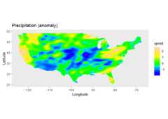
Further examples can be found in the vignette.
vignette("Solving_Linear_Mixed_Models")