
TheJMH package jointly models both mean trajectory andwithin-subject variability of the longitudinal biomarker together withthe (competing risks) survival outcome.
You can install the development version of JMH fromGitHub with:
# install.packages("devtools")devtools::install_github("shanpengli/JMH")TheJMH package comes with several simulated datasets.To fit a joint model, we useJMMLSM function.
library(JMH)#> Loading required package: survival#> Loading required package: nlme#> Loading required package: MASS#> Loading required package: statmoddata(ydata)data(cdata)## fit a joint modelfit<-JMMLSM(cdata = cdata,ydata = ydata,long.formula = Y~ Z1+ Z2+ Z3+ time,surv.formula =Surv(survtime, cmprsk)~ var1+ var2+ var3,variance.formula =~ Z1+ Z2+ Z3+ time,quadpoint =6,random =~1|ID,print.para =FALSE)fit#>#> Call:#> JMMLSM(cdata = cdata, ydata = ydata, long.formula = Y ~ Z1 + Z2 + Z3 + time, surv.formula = Surv(survtime, cmprsk) ~ var1 + var2 + var3, variance.formula = ~Z1 + Z2 + Z3 + time, random = ~1 | ID, quadpoint = 6, print.para = FALSE)#>#> Data Summary:#> Number of observations: 1353#> Number of groups: 200#>#> Proportion of competing risks:#> Risk 1 : 45.5 %#> Risk 2 : 32.5 %#>#> Numerical intergration:#> Method: adaptive Guass-Hermite quadrature#> Number of quadrature points: 6#>#> Model Type: joint modeling of longitudinal continuous and competing risks data with the presence of intra-individual variability#>#> Model summary:#> Longitudinal process: Mixed effects location scale model#> Event process: cause-specific Cox proportional hazard model with non-parametric baseline hazard#>#> Loglikelihood: -3621.603#>#> Fixed effects in mean of longitudinal submodel: Y ~ Z1 + Z2 + Z3 + time#>#> Estimate SE Z value p-val#> (Intercept) 4.85342 0.12451 38.97918 0.0000#> Z1 1.55235 0.16535 9.38841 0.0000#> Z2 1.93774 0.14598 13.27409 0.0000#> Z3 1.09289 0.05321 20.53796 0.0000#> time 4.01129 0.02978 134.71376 0.0000#>#> Fixed effects in variance of longitudinal submodel: log(sigma^2) ~ Z1 + Z2 + Z3 + time#>#> Estimate SE Z value p-val#> (Intercept) 0.50745 0.12838 3.95260 0.0001#> Z1 0.50509 0.16005 3.15590 0.0016#> Z2 -0.42508 0.13781 -3.08463 0.0020#> Z3 0.14405 0.04494 3.20563 0.0013#> time 0.09050 0.02422 3.73720 0.0002#>#> Survival sub-model fixed effects: Surv(survtime, cmprsk) ~ var1 + var2 + var3#>#> Estimate SE Z value p-val#> var1_1 1.09710 0.32647 3.36051 0.0008#> var2_1 0.19237 0.26154 0.73553 0.4620#> var3_1 0.49611 0.08908 5.56951 0.0000#>#> var1_2 -0.88311 0.33702 -2.62037 0.0088#> var2_2 0.80905 0.30127 2.68549 0.0072#> var3_2 0.20871 0.09312 2.24143 0.0250#>#> Association parameters:#> Estimate SE Z value p-val#> (Intercept)_1 0.97480 0.62808 1.55202 0.1207#> (Intercept)_2 -0.18580 0.47949 -0.38750 0.6984#> var_(Intercept)_1 0.50030 0.58190 0.85977 0.3899#> var_(Intercept)_2 -0.84481 0.52520 -1.60857 0.1077#>#>#> Random effects:#> Formula: ~1 | ID#> Estimate SE Z value p-val#> (Intercept) 0.49542 0.11339 4.36913 0.0000#> var_(Intercept) 0.45581 0.11129 4.09578 0.0000#> (Intercept):var_(Intercept) 0.26738 0.07854 3.40429 0.0007TheJMH package can make dynamic prediction given thelongitudinal history information. Below is a toy example for competingrisks data. Conditional cumulative incidence probabilities for eachfailure will be presented.
cnewdata<- cdata[cdata$ID%in%c(122,152), ]ynewdata<- ydata[ydata$ID%in%c(122,152), ]survfit<-survfitJMMLSM(fit,seed =100,ynewdata = ynewdata,cnewdata = cnewdata,u =seq(5.2,7.2,by =0.5),Last.time ="survtime",obs.time ="time",method ="GH")survfit#>#> Prediction of Conditional Probabilities of Event#> based on the adaptive Guass-Hermite quadrature rule with 6 quadrature points#> $`122`#> times CIF1 CIF2#> 1 5.069089 0.00000000 0.0000000#> 2 5.200000 0.05596021 0.0000000#> 3 5.700000 0.14584944 0.0000000#> 4 6.200000 0.33882152 0.0000000#> 5 6.700000 0.33882152 0.0000000#> 6 7.200000 0.33882152 0.2171424#>#> $`152`#> times CIF1 CIF2#> 1 5.133665 0.0000000 0.00000000#> 2 5.200000 0.0517717 0.00000000#> 3 5.700000 0.1357406 0.00000000#> 4 6.200000 0.3195265 0.00000000#> 5 6.700000 0.3195265 0.00000000#> 6 7.200000 0.3195265 0.06007945oldpar<-par(mfrow =c(2,2),mar =c(5,4,4,4))plot(survfit,include.y =TRUE)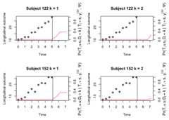
par(oldpar)If we assess the prediction accuracy of the fitted joint model usingBrier score as a calibration measure, we may runPEJMMLSMto calculate the Brier score.
PE<-PEJMMLSM(fit,seed =100,landmark.time =3,horizon.time =c(4:6),obs.time ="time",method ="GH",n.cv =3)#> The 1 th validation is done!#> The 2 th validation is done!#> The 3 th validation is done!summary(PE,error ="Brier")#>#> Expected Brier Score at the landmark time of 3#> based on 3 fold cross validation#> Horizon Time Brier Score 1 Brier Score 2#> 1 4 0.06369906 0.06194668#> 2 5 0.10838731 0.11052099#> 3 6 0.20187572 0.11613515An alternative tool is to runMAEQJMMLSM to calculatethe prediction error by comparing the predicted and empirical risksstratified on different risk groups based on quantile of the predictedrisks.
## evaluate prediction accuracy of fitted joint model using cross-validated mean absolute prediction errorMAEQ<-MAEQJMMLSM(fit,seed =100,landmark.time =3,horizon.time =c(4:6),obs.time ="time",method ="GH",n.cv =3)#> The 1 th validation is done!#> The 2 th validation is done!#> The 3 th validation is done!summary(MAEQ)#>#> Sum of absolute error across quintiles of predicted risk scores at the landmark time of 3#> based on 3 fold cross validation#> Horizon Time CIF1 CIF2#> 1 4 0.386 0.262#> 2 5 0.476 0.346#> 3 6 0.456 0.430Using area under the ROC curve (AUC) as a discrimination measure, wemay runAUCJMMLSM to calculate the AUC score.
AUC<-AUCJMMLSM(fit,seed =100,landmark.time =3,horizon.time =c(4:6),obs.time ="time",method ="GH",n.cv =3)#> The 1 th validation is done!#> The 2 th validation is done!#> The 3 th validation is done!summary(AUC)#>#> Expected AUC at the landmark time of 3#> based on 3 fold cross validation#> Horizon Time AUC1 AUC2#> 1 4 0.5502137 0.6839226#> 2 5 0.6182312 0.6523506#> 3 6 0.6103724 0.7065657