15 January, 2021
assess_reference_loo()This is an R package for performing genetic stock identification(GSI) and associated tasks. Additionally, it includes a method designedto diagnose and correct a bias recently documented in genetic stockidentification. The bias occurs when mixture proportion estimates aredesired for groups of populations (reporting units) and the number ofpopulations within each reporting unit are uneven.
In order to run C++ implementations of MCMC, rubias requires thepackage Rcpp (and now, also, RcppParallel for the baseline resamplingoption), which in turn requires an Rtools installation (if you are onWindows) or XCode (if you are on a Mac). After cloning into therepository with the above dependencies installed, build & reload thepackage to view further documentation.
The script “/R-main/coalescent_sim” was used to generate coalescentsimulations for bias correction validation. This is unnecessary fortesting the applicability of our methods to any particular dataset,which should be done usingassess_reference_loo() andassess_pb_bias_correction().coalescent_sim()creates simulated populations using thems coalescentsimulation program, available from the Hudson lab at UChicago, and theGSImulator andms2geno packages, available athttps://github.com/eriqande, and so requires moredependencies than the rest of the package.
The functions for conducting genetic mixture analysis and for doingsimulation assessment to predict the accuracy of a set of geneticmarkers for genetic stock identification require that genetic data beinput as a data frame in a specific format:
sample_type: a column telling whether the sample is areference sample or amixture sample.repunit: the reporting unit that anindividual/collection belongs to. This is required if sample_type isreference. And if sample_type ismixture thenrepunit must beNA.collection: for reference samples, the name of thepopulation that the individual is from. For mixture samples, this is thename of the particular sample (i.e. stratum or port that is to betreated together in space and time). This must be a character, not afactor.indiv a character vector with the ID of the fish. Thesemust be unique.rubias, we intended to allowboth therepunit and thecollection columns tobe either character vectors or factors. Having them as factors might bedesirable if, for example, a certain sort order of the collections orrepunits was desired.However at some point it became clear toEric that, given our approach to converting all the data to a C++ datastructure of integers, for rapid analyis, we would be exposing ourselvesto greater opportunities for bugginess by allowingrepunitandcollection to be factors. Accordingly, theymust be character vectors. If they are not,rubias will throw an error.Note: if youdo have a specific sort order for your collections or repunits, you canalways change them into factors after analysis withrubias.Additionally, you can keep extra columns in your original data frame(for examplerepunit_f orcollection_f) inwhich the repunits or the collections are stored as factors. See, forexample the data filealewife. Or you can just keep acharacter vector that has the sort order you would like, so as to use itwhen changing things to factors afterrubias analysis.(See, for instance,chinook_repunit_levels.)At the request of the good folks at ADFG, I introduced a few hacks toallow the input to include markers that are haploid (for example mtDNAhaplotypes). To denote a marker as haploid youstill give it twocolumns of data in your data frame, but the second column of thehaploid marker must be entirely NAs. Whenrubias isprocessing the data and it sees this, it assumes that the marker ishaploid and it treats it appropriately.
Note that if you have a diploid marker it typically does not makesense to mark one of the gene copies as missing and the other asnon-missing. Accordingly, if you have a diploid marker that records justone of the gene copies as missing in any individual, it is going tothrow an error. Likewise, if your haploid marker does not have everysingle individual with and NA at the second gene copy, then it’s alsogoing to throw an error.
Here are the meta data columns and the first two loci for eightindividuals in thechinook reference data set that comeswith the package:
library(tidyverse)# load up the tidyverse library, we will use it later...#> ── Attaching packages ─────────────────────────────────────── tidyverse 1.3.0 ──#> ✓ ggplot2 3.3.2 ✓ purrr 0.3.4#> ✓ tibble 3.0.4 ✓ dplyr 1.0.2#> ✓ tidyr 1.1.2 ✓ stringr 1.4.0#> ✓ readr 1.4.0 ✓ forcats 0.5.0#> ── Conflicts ────────────────────────────────────────── tidyverse_conflicts() ──#> x dplyr::filter() masks stats::filter()#> x dplyr::lag() masks stats::lag()library(rubias)head(chinook[,1:8])#> # A tibble: 6 x 8#> sample_type repunit collection indiv Ots_94857.232 Ots_94857.232.1#> <chr> <chr> <chr> <chr> <int> <int>#> 1 reference Centra… Feather_H… Feat… 2 2#> 2 reference Centra… Feather_H… Feat… 2 4#> 3 reference Centra… Feather_H… Feat… 2 4#> 4 reference Centra… Feather_H… Feat… 2 4#> 5 reference Centra… Feather_H… Feat… 2 2#> 6 reference Centra… Feather_H… Feat… 2 4#> # … with 2 more variables: Ots_102213.210 <int>, Ots_102213.210.1 <int>Here is the same for the mixture data frame that goes along with thatreference data set:
head(chinook_mix[,1:8])#> # A tibble: 6 x 8#> sample_type repunit collection indiv Ots_94857.232 Ots_94857.232.1#> <chr> <chr> <chr> <chr> <int> <int>#> 1 mixture <NA> rec2 T124… 4 2#> 2 mixture <NA> rec2 T124… 4 2#> 3 mixture <NA> rec2 T124… 4 4#> 4 mixture <NA> rec1 T124… 4 4#> 5 mixture <NA> rec1 T124… 2 2#> 6 mixture <NA> rec1 T124… 4 2#> # … with 2 more variables: Ots_102213.210 <int>, Ots_102213.210.1 <int>Sometimes, for a variety of reasons, an individual’s genotype mightappear more than once in a data set.rubias has a quick anddirty function to spot pairs of individuals that share a large number ofgenotypes. Clearly you only want to look at pairs that don’t have awhole lot of missing data, so one parameter is the fraction of loci thatare non-missing in either fish. In our experience with Fluidigm assays,if a fish is missing at > 10% of the SNPs, the remaining genotypesare likely to have a fairly high error rate. So, to look for matchingsamples, let’s require 85% of the genotypes to be non-missing in bothmembers of the pair. The last parameter is the fraction of non-missingloci at which the pair has the same genotype. We will set that to 0.94first. Here we see it in action:
# combine chinook and chinook_mix into one big data frame,# but drop the California_Coho collection because Coho all# have pretty much the same genotype at these loci!chinook_all<-bind_rows(chinook, chinook_mix)%>%filter(collection!="California_Coho")# then toss them into a function. This takes half a minute or so...matchy_pairs<-close_matching_samples(D = chinook_all,gen_start_col =5,min_frac_non_miss =0.85,min_frac_matching =0.94 )#> Summary Statistics:#>#> 9510 Individuals in Sample#>#> 91 Loci: AldB1.122, AldoB4.183, OTNAML12_1.SNP1, Ots_100884.287, Ots_101119.381, Ots_101704.143, Ots_102213.210, Ots_102414.395, Ots_102420.494, Ots_102457.132, Ots_102801.308, Ots_102867.609, Ots_103041.52, Ots_104063.132, Ots_104569.86, Ots_105105.613, Ots_105132.200, Ots_105401.325, Ots_105407.117, Ots_106499.70, Ots_106747.239, Ots_107074.284, Ots_107285.93, Ots_107806.821, Ots_108007.208, Ots_108390.329, Ots_108735.302, Ots_109693.392, Ots_110064.383, Ots_110201.363, Ots_110495.380, Ots_110551.64, Ots_111312.435, Ots_111666.408, Ots_111681.657, Ots_112301.43, Ots_112419.131, Ots_112820.284, Ots_112876.371, Ots_113242.216, Ots_113457.40, Ots_117043.255, Ots_117242.136, Ots_117432.409, Ots_118175.479, Ots_118205.61, Ots_118938.325, Ots_122414.56, Ots_123048.521, Ots_123921.111, Ots_124774.477, Ots_127236.62, Ots_128302.57, Ots_128693.461, Ots_128757.61, Ots_129144.472, Ots_129170.683, Ots_129458.451, Ots_130720.99, Ots_131460.584, Ots_131906.141, Ots_94857.232, Ots_96222.525, Ots_96500.180, Ots_97077.179, Ots_99550.204, Ots_ARNT.195, Ots_AsnRS.60, Ots_aspat.196, Ots_CD59.2, Ots_CD63, Ots_EP.529, Ots_GDH.81x, Ots_HSP90B.385, Ots_MHC1, Ots_mybp.85, Ots_myoD.364, Ots_Ots311.101x, Ots_PGK.54, Ots_Prl2, Ots_RFC2.558, Ots_SClkF2R2.135, Ots_SWS1op.182, Ots_TAPBP, Ots_u07.07.161, Ots_u07.49.290, Ots_u4.92, OTSBMP.2.SNP1, OTSTF1.SNP1, S71.336, unk_526#>#> 39 Reporting Units: CentralValleyfa, CentralValleysp, CentralValleywi, CaliforniaCoast, KlamathR, NCaliforniaSOregonCoast, RogueR, MidOregonCoast, NOregonCoast, WillametteR, DeschutesRfa, LColumbiaRfa, LColumbiaRsp, MidColumbiaRtule, UColumbiaRsufa, MidandUpperColumbiaRsp, SnakeRfa, SnakeRspsu, NPugetSound, WashingtonCoast, SPugetSound, LFraserR, LThompsonR, EVancouverIs, WVancouverIs, MSkeenaR, MidSkeenaR, LSkeenaR, SSEAlaska, NGulfCoastAlsekR, NGulfCoastKarlukR, TakuR, NSEAlaskaChilkatR, NGulfCoastSitukR, CopperR, SusitnaR, LKuskokwimBristolBay, MidYukon#>#> 68 Collections: Feather_H_sp, Butte_Cr_Sp, Mill_Cr_sp, Deer_Cr_sp, UpperSacramento_R_sp, Feather_H_fa, Butte_Cr_fa, Mill_Cr_fa, Deer_Cr_fa, Mokelumne_R_fa, Battle_Cr, Sacramento_R_lf, Sacramento_H, Eel_R, Russian_R, Klamath_IGH_fa, Trinity_H_sp, Smith_R, Chetco_R, Cole_Rivers_H, Applegate_Cr, Coquille_R, Umpqua_sp, Nestucca_H, Siuslaw_R, Alsea_R, Nehalem_R, Siletz_R, N_Santiam_H, McKenzie_H, L_Deschutes_R, Cowlitz_H_fa, Cowlitz_H_sp, Kalama_H_sp, Spring_Cr_H, Hanford_Reach, PriestRapids_H, Wells_H, Wenatchee_R, CleElum, Lyons_Ferry_H, Rapid_R_H, McCall_H, Kendall_H_sp, Forks_Cr_H, Soos_H, Marblemount_H_sp, QuinaltLake_f, Harris_R, Birkenhead_H, Spius_H, Big_Qual_H, Robertson_H, Morice_R, Kitwanga_R, L_Kalum_R, LPW_Unuk_R, Goat_Cr, Karluk_R, LittleTatsamenie, Tahini_R, Situk_R, Sinona_Ck, Montana_Ck, George_R, Kanektok_R, Togiak_R, Kantishna_R#>#> 3.85% of allelic data identified as missing# see that that looks like:matchy_pairs%>%arrange(desc(num_non_miss),desc(num_match))#> # A tibble: 33 x 10#> num_non_miss num_match indiv_1 indiv_2 collection_1 collection_2#> <int> <int> <chr> <chr> <chr> <chr>#> 1 91 91 T124864 T124866 rec3 rec1#> 2 91 91 T124864 T125335 rec3 rec3#> 3 91 91 T124866 T125335 rec1 rec3#> 4 91 91 T126402 T126403 rec2 rec2#> 5 91 90 Mill_C… Mill_C… Mill_Cr_sp Mill_Cr_sp#> 6 91 90 Cole_R… Cole_R… Cole_Rivers… Cole_Rivers…#> 7 91 90 Cole_R… Cole_R… Cole_Rivers… Cole_Rivers…#> 8 91 90 Umpqua… Umpqua… Umpqua_sp Umpqua_sp#> 9 91 90 Umpqua… Umpqua… Umpqua_sp Umpqua_sp#> 10 91 90 T125044 T125337 rec2 rec1#> # … with 23 more rows, and 4 more variables: sample_type_1 <chr>,#> # repunit_1 <chr>, sample_type_2 <chr>, repunit_2 <chr>Check that out. This reveals 33 pairs in the data set that are likelyduplicate samples.
If we reduce the min_frac_matching, we get more matches, but theseare very unlikely to be the same individual, unless genotyping errorrates are very high.
# then toss them into a function. This takes half a minute or so...matchy_pairs2<-close_matching_samples(D = chinook_all,gen_start_col =5,min_frac_non_miss =0.85,min_frac_matching =0.85 )#> Summary Statistics:#>#> 9510 Individuals in Sample#>#> 91 Loci: AldB1.122, AldoB4.183, OTNAML12_1.SNP1, Ots_100884.287, Ots_101119.381, Ots_101704.143, Ots_102213.210, Ots_102414.395, Ots_102420.494, Ots_102457.132, Ots_102801.308, Ots_102867.609, Ots_103041.52, Ots_104063.132, Ots_104569.86, Ots_105105.613, Ots_105132.200, Ots_105401.325, Ots_105407.117, Ots_106499.70, Ots_106747.239, Ots_107074.284, Ots_107285.93, Ots_107806.821, Ots_108007.208, Ots_108390.329, Ots_108735.302, Ots_109693.392, Ots_110064.383, Ots_110201.363, Ots_110495.380, Ots_110551.64, Ots_111312.435, Ots_111666.408, Ots_111681.657, Ots_112301.43, Ots_112419.131, Ots_112820.284, Ots_112876.371, Ots_113242.216, Ots_113457.40, Ots_117043.255, Ots_117242.136, Ots_117432.409, Ots_118175.479, Ots_118205.61, Ots_118938.325, Ots_122414.56, Ots_123048.521, Ots_123921.111, Ots_124774.477, Ots_127236.62, Ots_128302.57, Ots_128693.461, Ots_128757.61, Ots_129144.472, Ots_129170.683, Ots_129458.451, Ots_130720.99, Ots_131460.584, Ots_131906.141, Ots_94857.232, Ots_96222.525, Ots_96500.180, Ots_97077.179, Ots_99550.204, Ots_ARNT.195, Ots_AsnRS.60, Ots_aspat.196, Ots_CD59.2, Ots_CD63, Ots_EP.529, Ots_GDH.81x, Ots_HSP90B.385, Ots_MHC1, Ots_mybp.85, Ots_myoD.364, Ots_Ots311.101x, Ots_PGK.54, Ots_Prl2, Ots_RFC2.558, Ots_SClkF2R2.135, Ots_SWS1op.182, Ots_TAPBP, Ots_u07.07.161, Ots_u07.49.290, Ots_u4.92, OTSBMP.2.SNP1, OTSTF1.SNP1, S71.336, unk_526#>#> 39 Reporting Units: CentralValleyfa, CentralValleysp, CentralValleywi, CaliforniaCoast, KlamathR, NCaliforniaSOregonCoast, RogueR, MidOregonCoast, NOregonCoast, WillametteR, DeschutesRfa, LColumbiaRfa, LColumbiaRsp, MidColumbiaRtule, UColumbiaRsufa, MidandUpperColumbiaRsp, SnakeRfa, SnakeRspsu, NPugetSound, WashingtonCoast, SPugetSound, LFraserR, LThompsonR, EVancouverIs, WVancouverIs, MSkeenaR, MidSkeenaR, LSkeenaR, SSEAlaska, NGulfCoastAlsekR, NGulfCoastKarlukR, TakuR, NSEAlaskaChilkatR, NGulfCoastSitukR, CopperR, SusitnaR, LKuskokwimBristolBay, MidYukon#>#> 68 Collections: Feather_H_sp, Butte_Cr_Sp, Mill_Cr_sp, Deer_Cr_sp, UpperSacramento_R_sp, Feather_H_fa, Butte_Cr_fa, Mill_Cr_fa, Deer_Cr_fa, Mokelumne_R_fa, Battle_Cr, Sacramento_R_lf, Sacramento_H, Eel_R, Russian_R, Klamath_IGH_fa, Trinity_H_sp, Smith_R, Chetco_R, Cole_Rivers_H, Applegate_Cr, Coquille_R, Umpqua_sp, Nestucca_H, Siuslaw_R, Alsea_R, Nehalem_R, Siletz_R, N_Santiam_H, McKenzie_H, L_Deschutes_R, Cowlitz_H_fa, Cowlitz_H_sp, Kalama_H_sp, Spring_Cr_H, Hanford_Reach, PriestRapids_H, Wells_H, Wenatchee_R, CleElum, Lyons_Ferry_H, Rapid_R_H, McCall_H, Kendall_H_sp, Forks_Cr_H, Soos_H, Marblemount_H_sp, QuinaltLake_f, Harris_R, Birkenhead_H, Spius_H, Big_Qual_H, Robertson_H, Morice_R, Kitwanga_R, L_Kalum_R, LPW_Unuk_R, Goat_Cr, Karluk_R, LittleTatsamenie, Tahini_R, Situk_R, Sinona_Ck, Montana_Ck, George_R, Kanektok_R, Togiak_R, Kantishna_R#>#> 3.85% of allelic data identified as missing# see that that looks like:matchy_pairs2%>%arrange(desc(num_non_miss),desc(num_match))#> # A tibble: 46 x 10#> num_non_miss num_match indiv_1 indiv_2 collection_1 collection_2#> <int> <int> <chr> <chr> <chr> <chr>#> 1 91 91 T124864 T124866 rec3 rec1#> 2 91 91 T124864 T125335 rec3 rec3#> 3 91 91 T124866 T125335 rec1 rec3#> 4 91 91 T126402 T126403 rec2 rec2#> 5 91 90 Mill_C… Mill_C… Mill_Cr_sp Mill_Cr_sp#> 6 91 90 Cole_R… Cole_R… Cole_Rivers… Cole_Rivers…#> 7 91 90 Cole_R… Cole_R… Cole_Rivers… Cole_Rivers…#> 8 91 90 Umpqua… Umpqua… Umpqua_sp Umpqua_sp#> 9 91 90 Umpqua… Umpqua… Umpqua_sp Umpqua_sp#> 10 91 90 T125044 T125337 rec2 rec1#> # … with 36 more rows, and 4 more variables: sample_type_1 <chr>,#> # repunit_1 <chr>, sample_type_2 <chr>, repunit_2 <chr>A more principled approach would be to use the allele frequencies ineach collection and take a likelihood based approach, but this isadequate for finding obvious duplicates.
In some cases, you might know (more or less unambiguously) the originof some fish in a particular mixture sample. For example, if 10% of theindividuals in a mixture carried coded wire tags, then you would want toinclude them in the sample, but make sure that their collections oforigin were hard-coded to be what the CWTs said. Another scenario inwhich this might occur is when the genetic data were used forparentage-based tagging of the individuals in the mixture sample. Inthat case, some individuals might be placed with very high confidence toparents. Then, they should be included in the mixture as having comefrom a known collection. The folks at the DFO in Nanaimo, Canada aredoing an amazing job with PBT and wondered if rubias could be modifiedto deal with the latter situation.
We’ve made some small additions to accommodate this. rubias does notdo any actual inference of parentage, but if you know the origin of somefish in the mixture, that can be included in the rubias analysis. Theway you do this with the functioninfer_mixture() is toinclude a column calledknown_collection in both thereference data frame and the mixture data frame. In the reference dataframe,known_collection should just be a copy of thecollection column. However, in the mixture data frame eachentry inknown_collection should be the collection that theindividual is known to be from (i.e. using parentage inference or aCWT), or, if the individual is not known to be from any collection, itshould be NA. Note that the names of the collections inknown_collection must match those found in thecollection column in the reference data set.
These modifications are not allowed for the parametric bootstrap (PB)method ininfer_mixture().
This is done with theinfer_mixture function. In theexample datachinook_mix our data consist of fish caught inthree different fisheries,rec1,rec2, andrec3 as denoted in the collection column. Each of thosecollections is treated as a separate sample, getting its own mixingproportion estimate. This is how it is run with the default options:
mix_est<-infer_mixture(reference = chinook,mixture = chinook_mix,gen_start_col =5)#> Collating data; compiling reference allele frequencies, etc. time: 1.64 seconds#> Computing reference locus specific means and variances for computing mixture z-scores time: 0.24 seconds#> Working on mixture collection: rec2 with 772 individuals#> calculating log-likelihoods of the mixture individuals. time: 0.12 seconds#> performing 2000 total sweeps, 100 of which are burn-in and will not be used in computing averages in method "MCMC" time: 0.63 seconds#> tidying output into a tibble. time: 0.25 seconds#> Working on mixture collection: rec1 with 743 individuals#> calculating log-likelihoods of the mixture individuals. time: 0.11 seconds#> performing 2000 total sweeps, 100 of which are burn-in and will not be used in computing averages in method "MCMC" time: 0.61 seconds#> tidying output into a tibble. time: 0.26 seconds#> Working on mixture collection: rec3 with 741 individuals#> calculating log-likelihoods of the mixture individuals. time: 0.11 seconds#> performing 2000 total sweeps, 100 of which are burn-in and will not be used in computing averages in method "MCMC" time: 0.60 seconds#> tidying output into a tibble. time: 0.29 secondsThe result comes back as a list of four tidy data frames:
mixing_proportions: the mixing proportions. The columnpi holds the estimated mixing proportion for eachcollection.indiv_posteriors: this holds, for each individual, theposterior means of group membership in each collection. ColumnPofZ holds those values. Columnlog_likelihoodholds the log of the probability of the individuals genotype given it isfrom the collection. Also included aren_non_miss_loci andn_miss_loci which are the number of observed loci and thenumber of missing loci at the individual. A list columnmissing_loci contains vectors with the indices (and thenames) of the loci that are missing in that individual. It also includesa columnz_score which can be used to diagnose fish thatdon’t belong to any samples in the reference data base (see below).mix_prop_traces: MCMC traces of the mixing proportionsfor each collection. You will use these if you want to make densityestimates of the posterior distribution of the mixing proportions or ifyou want to compute credible intervals.bootstrapped_proportions: This is NULL in the aboveexample, but if we had chosenmethod = "PB" then this wouldbe a tibble of bootstrap-corrected reporting unit mixingproportions.These data frames look like this:
lapply(mix_est, head)#> $mixing_proportions#> # A tibble: 6 x 4#> mixture_collection repunit collection pi#> <chr> <chr> <chr> <dbl>#> 1 rec2 CentralValleyfa Feather_H_sp 0.0781#> 2 rec2 CentralValleysp Butte_Cr_Sp 0.0000448#> 3 rec2 CentralValleysp Mill_Cr_sp 0.0000457#> 4 rec2 CentralValleysp Deer_Cr_sp 0.0000509#> 5 rec2 CentralValleysp UpperSacramento_R_sp 0.000310#> 6 rec2 CentralValleyfa Feather_H_fa 0.153#>#> $indiv_posteriors#> # A tibble: 6 x 10#> mixture_collect… indiv repunit collection PofZ log_likelihood z_score#> <chr> <chr> <chr> <chr> <dbl> <dbl> <dbl>#> 1 rec2 T124… Centra… Feather_H… 1.80e-28 -137. -13.1#> 2 rec2 T124… Centra… Feather_H… 1.01e-27 -136. -12.6#> 3 rec2 T124… Centra… Butte_Cr_… 1.57e-24 -130. -10.5#> 4 rec2 T124… Centra… Mill_Cr_fa 6.76e-30 -135. -11.8#> 5 rec2 T124… Centra… Deer_Cr_fa 1.49e-28 -134. -11.6#> 6 rec2 T124… Centra… Mokelumne… 1.91e-27 -134. -12.3#> # … with 3 more variables: n_non_miss_loci <int>, n_miss_loci <int>,#> # missing_loci <list>#>#> $mix_prop_traces#> # A tibble: 6 x 5#> mixture_collection sweep repunit collection pi#> <chr> <int> <chr> <chr> <dbl>#> 1 rec2 0 CentralValleyfa Feather_H_sp 0.0145#> 2 rec2 0 CentralValleysp Butte_Cr_Sp 0.0145#> 3 rec2 0 CentralValleysp Mill_Cr_sp 0.0145#> 4 rec2 0 CentralValleysp Deer_Cr_sp 0.0145#> 5 rec2 0 CentralValleysp UpperSacramento_R_sp 0.0145#> 6 rec2 0 CentralValleyfa Feather_H_fa 0.0145#>#> $bootstrapped_proportions#> # A tibble: 0 x 0In some cases there might be a reason to explicitly set theparameters of the Dirichlet prior on the mixing proportions of thecollections. For a contrived example, we could imagine that we wanted aDirichlet prior with all parameters equal to 1/(# of collections),except for the parameters for all the Central Valley Fall Runpopulations, to which we would like to assign Dirichlet parameters of 2.That can be accomplished with thepi_prior argument to theinfer_mixture() function, which will let you pass in atibble in which one column named “collection” gives the collection, andthe other column, named “pi_param” gives the desired parameter.
Here we construct that kind of input:
prior_tibble<- chinook%>%count(repunit, collection)%>%filter(repunit=="CentralValleyfa")%>%select(collection)%>%mutate(pi_param =2)# see what it looks like:prior_tibble#> # A tibble: 8 x 2#> collection pi_param#> <chr> <dbl>#> 1 Battle_Cr 2#> 2 Butte_Cr_fa 2#> 3 Deer_Cr_fa 2#> 4 Feather_H_fa 2#> 5 Feather_H_sp 2#> 6 Mill_Cr_fa 2#> 7 Mokelumne_R_fa 2#> 8 Sacramento_R_lf 2Then we can run that in infer_mixture():
set.seed(12)mix_est_with_prior<-infer_mixture(reference = chinook,mixture = chinook_mix,gen_start_col =5,pi_prior = prior_tibble)#> Collating data; compiling reference allele frequencies, etc. time: 1.56 seconds#> Computing reference locus specific means and variances for computing mixture z-scores time: 0.24 seconds#> Working on mixture collection: rec2 with 772 individuals#> Joining, by = "collection"#> calculating log-likelihoods of the mixture individuals. time: 0.12 seconds#> performing 2000 total sweeps, 100 of which are burn-in and will not be used in computing averages in method "MCMC" time: 0.62 seconds#> tidying output into a tibble. time: 0.25 seconds#> Working on mixture collection: rec1 with 743 individuals#> Joining, by = "collection"#> calculating log-likelihoods of the mixture individuals. time: 0.11 seconds#> performing 2000 total sweeps, 100 of which are burn-in and will not be used in computing averages in method "MCMC" time: 0.61 seconds#> tidying output into a tibble. time: 0.27 seconds#> Working on mixture collection: rec3 with 741 individuals#> Joining, by = "collection"#> calculating log-likelihoods of the mixture individuals. time: 0.11 seconds#> performing 2000 total sweeps, 100 of which are burn-in and will not be used in computing averages in method "MCMC" time: 0.59 seconds#> tidying output into a tibble. time: 0.28 secondsand now, for fun, we can compare the results for the mixingproportions of different collections there with and without the priorfor the mixture collection rec1:
comp_mix_ests<-list(`pi (default prior)`= mix_est$mixing_proportions,`pi (cv fall gets 2s prior)`= mix_est_with_prior$mixing_proportions)%>%bind_rows(.id ="prior_type")%>%filter(mixture_collection=="rec1")%>%select(prior_type, repunit, collection, pi)%>%spread(prior_type, pi)%>%mutate(coll_group =ifelse(repunit=="CentralValleyfa","CV_fall","Not_CV_fall"))ggplot(comp_mix_ests,aes(x =`pi (default prior)`,y =`pi (cv fall gets 2s prior)`,colour = coll_group ))+geom_point()+geom_abline(slope =1,intercept =0,linetype ="dashed")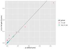
Yep, slightly different than before. Let’s look at the sums ofeverything:
comp_mix_ests%>%group_by(coll_group)%>%summarise(with_explicit_prior =sum(`pi (cv fall gets 2s prior)`),with_default_prior =sum(`pi (default prior)`))#> `summarise()` ungrouping output (override with `.groups` argument)#> # A tibble: 2 x 3#> coll_group with_explicit_prior with_default_prior#> <chr> <dbl> <dbl>#> 1 CV_fall 0.824 0.819#> 2 Not_CV_fall 0.176 0.181We see that for the most part this change to the prior changed thedistribution of fish into different collections within the CentralValley Fall reporting unit. This is not suprising—it is very hard totell apart fish from those different collections. However, it did notgreatly change the estimated proportion of the whole reporting unit.This also turns out to make sense if you consider the effect that theextra weight in the prior will have.
This is a simple operation in thetidyverse:
# for mixing proportionsrep_mix_ests<- mix_est$mixing_proportions%>%group_by(mixture_collection, repunit)%>%summarise(repprop =sum(pi))# adding mixing proportions over collections in the repunit#> `summarise()` regrouping output by 'mixture_collection' (override with `.groups` argument)# for individuals posteriorsrep_indiv_ests<- mix_est$indiv_posteriors%>%group_by(mixture_collection, indiv, repunit)%>%summarise(rep_pofz =sum(PofZ))#> `summarise()` regrouping output by 'mixture_collection', 'indiv' (override with `.groups` argument)The full MCMC output for the mixing proportions is available bydefault in the field$mix_prop_traces. This can be used toobtain an estimate of the posterior density of the mixingproportions.
Here we plot kernel density estimates for the 6 most abundantrepunits from therec1 fishery:
# find the top 6 most abundant:top6<- rep_mix_ests%>%filter(mixture_collection=="rec1")%>%arrange(desc(repprop))%>%slice(1:6)# check how many MCMC sweeps were done:nsweeps<-max(mix_est$mix_prop_traces$sweep)# keep only rec1, then discard the first 200 sweeps as burn-in,# and then aggregate over reporting units# and then keep only the top6 from abovetrace_subset<- mix_est$mix_prop_traces%>%filter(mixture_collection=="rec1", sweep>200)%>%group_by(sweep, repunit)%>%summarise(repprop =sum(pi))%>%filter(repunit%in% top6$repunit)#> `summarise()` regrouping output by 'sweep' (override with `.groups` argument)# now we can plot those:ggplot(trace_subset,aes(x = repprop,colour = repunit))+geom_density()
Following on from the above example, we will usetrace_subset to compute the equal-tail 95% credibleintervals for the 6 most abundant reporting units in therec1 fishery:
top6_cis<- trace_subset%>%group_by(repunit)%>%summarise(loCI =quantile(repprop,probs =0.025),hiCI =quantile(repprop,probs =0.975))#> `summarise()` ungrouping output (override with `.groups` argument)top6_cis#> # A tibble: 6 x 3#> repunit loCI hiCI#> <chr> <dbl> <dbl>#> 1 CaliforniaCoast 1.84e- 2 0.0443#> 2 CentralValleyfa 7.88e- 1 0.847#> 3 KlamathR 4.98e- 2 0.0875#> 4 NCaliforniaSOregonCoast 2.99e- 3 0.0184#> 5 RogueR 4.37e- 2 0.0826#> 6 SnakeRfa 2.56e-89 0.0119Sometimes totally unexpected things happen. One situation we saw inthe California Chinook fishery was samples coming to us that wereactually coho salmon. Before we included coho salmon in the referencesample, these coho always assigned quite strongly to Alaska populationsof Chinook, even though they don’t really look like Chinook at all.
In this case, it is useful to look at the raw log-likelihood valuescomputed for the individual, rather than the scaled posteriorprobabilities. Because aberrantly low values of the genotypelog-likelihood can indicate that there is something wrong. However, theraw likelihood that you get will depend on the number of missing loci,etc.rubias deals with this by computing az-scorefor each fish. The Z-score is the Z statistic obtained from the fish’slog-likelihood (by subtracting from it the expected log-likelihood anddividing by the expected standard deviation).rubias’simplementation of the z-score accounts for the pattern of missing data,but it does this without all the simulation thatgsi_simdoes. This makes it much, much, faster—fast enough that we can computeit be default for every fish and every population.
Here, we will look at the z-score computed for each fish to thepopulation with the highest posterior. (It is worth noting that youwouldnever want to use the z-score to assign fish todifferent populations—it is only there to decide whether it looks likeit might not have actually come from the population that it was assignedto, or any other population in the reference data set.)
# get the maximum-a-posteriori population for each individualmap_rows<- mix_est$indiv_posteriors%>%group_by(indiv)%>%top_n(1, PofZ)%>%ungroup()If everything is kosher, then we expect that the z-scores we see willbe roughly normally distributed. We can compare the distribution ofz-scores we see with a bunch of simulated normal random variables.
normo<-tibble(z_score =rnorm(1e06))ggplot(map_rows,aes(x = z_score))+geom_density(colour ="blue")+geom_density(data = normo,colour ="black")
The normal density is in black and the distribution of our observedz_scores is in blue. They fit reasonably well, suggesting that there isnot too much weird stuff going on overall. (That is good!)
The z_score statistic is most useful as a check for individuals. Itis intended to be a quick way to identify aberrant individuals. If yousee a z-score to the maximum-a-posteriori population for an individualin your mixture sample that is considerably less than z_scores you sawin the reference, then you might infer that the individual doesn’tactually fit any of the populations in the reference well.
Here I include a small, contrived example. We use thesmall_chinook data set so that it goes fast.
First, we analyze the data with no fish in the mixture of knowncollection
no_kc<-infer_mixture(small_chinook_ref, small_chinook_mix,gen_start_col =5)#> Collating data; compiling reference allele frequencies, etc. time: 0.20 seconds#> Computing reference locus specific means and variances for computing mixture z-scores time: 0.02 seconds#> Working on mixture collection: rec3 with 29 individuals#> calculating log-likelihoods of the mixture individuals. time: 0.01 seconds#> performing 2000 total sweeps, 100 of which are burn-in and will not be used in computing averages in method "MCMC" time: 0.03 seconds#> tidying output into a tibble. time: 0.03 seconds#> Working on mixture collection: rec1 with 36 individuals#> calculating log-likelihoods of the mixture individuals. time: 0.01 seconds#> performing 2000 total sweeps, 100 of which are burn-in and will not be used in computing averages in method "MCMC" time: 0.03 seconds#> tidying output into a tibble. time: 0.03 seconds#> Working on mixture collection: rec2 with 35 individuals#> calculating log-likelihoods of the mixture individuals. time: 0.01 seconds#> performing 2000 total sweeps, 100 of which are burn-in and will not be used in computing averages in method "MCMC" time: 0.03 seconds#> tidying output into a tibble. time: 0.03 secondsAnd look at the results for the mixing proportions:
no_kc$mixing_proportions%>%arrange(mixture_collection,desc(pi))#> # A tibble: 18 x 4#> mixture_collection repunit collection pi#> <chr> <chr> <chr> <dbl>#> 1 rec1 CentralValleyfa Feather_H_fa 0.849#> 2 rec1 CentralValleysp Deer_Cr_sp 0.0508#> 3 rec1 CaliforniaCoast Eel_R 0.0400#> 4 rec1 KlamathR Klamath_IGH_fa 0.0305#> 5 rec1 MidOregonCoast Umpqua_sp 0.0252#> 6 rec1 CentralValleywi Sacramento_H 0.00463#> 7 rec2 CentralValleyfa Feather_H_fa 0.809#> 8 rec2 KlamathR Klamath_IGH_fa 0.103#> 9 rec2 MidOregonCoast Umpqua_sp 0.0733#> 10 rec2 CentralValleysp Deer_Cr_sp 0.00550#> 11 rec2 CaliforniaCoast Eel_R 0.00479#> 12 rec2 CentralValleywi Sacramento_H 0.00474#> 13 rec3 CentralValleyfa Feather_H_fa 0.839#> 14 rec3 CaliforniaCoast Eel_R 0.0714#> 15 rec3 MidOregonCoast Umpqua_sp 0.0496#> 16 rec3 KlamathR Klamath_IGH_fa 0.0262#> 17 rec3 CentralValleysp Deer_Cr_sp 0.00875#> 18 rec3 CentralValleywi Sacramento_H 0.00542Now, we will do the same analysis, but pretend that we know that thefirst 8 of the 36 fish in fishery rec1 are from the Deer_Cr_spcollection.
First we have to add the known_collection column to thereference.
# make reference file that includes the known_collection columnkc_ref<- small_chinook_ref%>%mutate(known_collection = collection)%>%select(known_collection,everything())# see what that looks likekc_ref[1:10,1:8]#> # A tibble: 10 x 8#> known_collection sample_type repunit collection indiv Ots_94857.232#> <chr> <chr> <chr> <chr> <chr> <int>#> 1 Deer_Cr_sp reference Centra… Deer_Cr_sp Deer… 2#> 2 Deer_Cr_sp reference Centra… Deer_Cr_sp Deer… 2#> 3 Deer_Cr_sp reference Centra… Deer_Cr_sp Deer… 2#> 4 Deer_Cr_sp reference Centra… Deer_Cr_sp Deer… 4#> 5 Deer_Cr_sp reference Centra… Deer_Cr_sp Deer… 2#> 6 Deer_Cr_sp reference Centra… Deer_Cr_sp Deer… 4#> 7 Deer_Cr_sp reference Centra… Deer_Cr_sp Deer… 2#> 8 Deer_Cr_sp reference Centra… Deer_Cr_sp Deer… 4#> 9 Deer_Cr_sp reference Centra… Deer_Cr_sp Deer… 2#> 10 Deer_Cr_sp reference Centra… Deer_Cr_sp Deer… 2#> # … with 2 more variables: Ots_94857.232.1 <int>, Ots_102213.210 <int>Then we add the known collection column to the mixture. We start outmaking it all NAs, and then we change that to Deer_Cr_sp for 8 of therec1 fish:
kc_mix<- small_chinook_mix%>%mutate(known_collection =NA)%>%select(known_collection,everything())kc_mix$known_collection[kc_mix$collection=="rec1"][1:8]<-"Deer_Cr_sp"# here is what that looks like now (dropping most of the genetic data columns)kc_mix[1:20,1:7]#> # A tibble: 20 x 7#> known_collection sample_type repunit collection indiv Ots_94857.232#> <chr> <chr> <chr> <chr> <chr> <int>#> 1 <NA> mixture <NA> rec3 T125… 4#> 2 Deer_Cr_sp mixture <NA> rec1 T127… 4#> 3 <NA> mixture <NA> rec2 T124… 4#> 4 <NA> mixture <NA> rec2 T127… 2#> 5 <NA> mixture <NA> rec3 T127… 4#> 6 Deer_Cr_sp mixture <NA> rec1 T127… 4#> 7 <NA> mixture <NA> rec3 T124… 4#> 8 Deer_Cr_sp mixture <NA> rec1 T126… 2#> 9 <NA> mixture <NA> rec3 T125… 4#> 10 Deer_Cr_sp mixture <NA> rec1 T127… 4#> 11 Deer_Cr_sp mixture <NA> rec1 T127… 2#> 12 Deer_Cr_sp mixture <NA> rec1 T127… 2#> 13 <NA> mixture <NA> rec2 T126… 4#> 14 <NA> mixture <NA> rec3 T126… 4#> 15 <NA> mixture <NA> rec2 T125… 4#> 16 Deer_Cr_sp mixture <NA> rec1 T126… 4#> 17 <NA> mixture <NA> rec2 T124… 4#> 18 <NA> mixture <NA> rec3 T124… 2#> 19 Deer_Cr_sp mixture <NA> rec1 T124… 4#> 20 <NA> mixture <NA> rec3 T125… 2#> # … with 1 more variable: Ots_94857.232.1 <int>And now we can do the mixture analysis:
# note that the genetic data start in column 6 nowwith_kc<-infer_mixture(kc_ref, kc_mix,6)#> Collating data; compiling reference allele frequencies, etc. time: 0.20 seconds#> Computing reference locus specific means and variances for computing mixture z-scores time: 0.02 seconds#> Working on mixture collection: rec3 with 29 individuals#> calculating log-likelihoods of the mixture individuals. time: 0.01 seconds#> performing 2000 total sweeps, 100 of which are burn-in and will not be used in computing averages in method "MCMC" time: 0.03 seconds#> tidying output into a tibble. time: 0.03 seconds#> Working on mixture collection: rec1 with 36 individuals#> calculating log-likelihoods of the mixture individuals. time: 0.01 seconds#> performing 2000 total sweeps, 100 of which are burn-in and will not be used in computing averages in method "MCMC" time: 0.03 seconds#> tidying output into a tibble. time: 0.03 seconds#> Working on mixture collection: rec2 with 35 individuals#> calculating log-likelihoods of the mixture individuals. time: 0.01 seconds#> performing 2000 total sweeps, 100 of which are burn-in and will not be used in computing averages in method "MCMC" time: 0.03 seconds#> tidying output into a tibble. time: 0.03 secondsAnd, when we look at the estimated proportions, we see that for rec1they reflect the fact that 8 of those fish were singled out as knownfish from Deer_Ck_sp:
with_kc$mixing_proportions%>%arrange(mixture_collection,desc(pi))#> # A tibble: 18 x 4#> mixture_collection repunit collection pi#> <chr> <chr> <chr> <dbl>#> 1 rec1 CentralValleyfa Feather_H_fa 0.546#> 2 rec1 CentralValleysp Deer_Cr_sp 0.355#> 3 rec1 CaliforniaCoast Eel_R 0.0411#> 4 rec1 KlamathR Klamath_IGH_fa 0.0318#> 5 rec1 MidOregonCoast Umpqua_sp 0.0220#> 6 rec1 CentralValleywi Sacramento_H 0.00438#> 7 rec2 CentralValleyfa Feather_H_fa 0.806#> 8 rec2 KlamathR Klamath_IGH_fa 0.104#> 9 rec2 MidOregonCoast Umpqua_sp 0.0732#> 10 rec2 CentralValleysp Deer_Cr_sp 0.00688#> 11 rec2 CaliforniaCoast Eel_R 0.00551#> 12 rec2 CentralValleywi Sacramento_H 0.00456#> 13 rec3 CentralValleyfa Feather_H_fa 0.835#> 14 rec3 CaliforniaCoast Eel_R 0.0732#> 15 rec3 MidOregonCoast Umpqua_sp 0.0494#> 16 rec3 KlamathR Klamath_IGH_fa 0.0281#> 17 rec3 CentralValleysp Deer_Cr_sp 0.00883#> 18 rec3 CentralValleywi Sacramento_H 0.00565The output frominfer_mixture() in this case can be usedjust like it was before without known individuals in the baseline.
The default model inrubias is a conditional model inwhich inference is done with the baseline allele counts fixed. In afully Bayesian version, fish from within the mixture that are allocated(on any particular step of the MCMC) to one of the reference sampleshave their alleles added to that reference sample, thus (one hopes)refining the estimate of allele frequencies in that sample. This is morecomputationally intensive, and, is done using parallel computation, bydefault running one thread for every core on your machine.
The basic way to invoke the fully Bayesian model is to use theinfer_mixture function with themethod optionset to “BR”. For example:
full_model_results<-infer_mixture(reference = chinook,mixture = chinook_mix,gen_start_col =5,method ="BR" )More details about different options for working with the fullyBayesian model are available in the vignette about the fully Bayesianmodel.
A standard analysis in molecular ecology is to assign individuals inthe reference back to the collections in the reference using aleave-one-out procedure. This is taken care of by theself_assign() function.
sa_chinook<-self_assign(reference = chinook,gen_start_col =5)#> Summary Statistics:#>#> 7301 Individuals in Sample#>#> 91 Loci: AldB1.122, AldoB4.183, OTNAML12_1.SNP1, Ots_100884.287, Ots_101119.381, Ots_101704.143, Ots_102213.210, Ots_102414.395, Ots_102420.494, Ots_102457.132, Ots_102801.308, Ots_102867.609, Ots_103041.52, Ots_104063.132, Ots_104569.86, Ots_105105.613, Ots_105132.200, Ots_105401.325, Ots_105407.117, Ots_106499.70, Ots_106747.239, Ots_107074.284, Ots_107285.93, Ots_107806.821, Ots_108007.208, Ots_108390.329, Ots_108735.302, Ots_109693.392, Ots_110064.383, Ots_110201.363, Ots_110495.380, Ots_110551.64, Ots_111312.435, Ots_111666.408, Ots_111681.657, Ots_112301.43, Ots_112419.131, Ots_112820.284, Ots_112876.371, Ots_113242.216, Ots_113457.40, Ots_117043.255, Ots_117242.136, Ots_117432.409, Ots_118175.479, Ots_118205.61, Ots_118938.325, Ots_122414.56, Ots_123048.521, Ots_123921.111, Ots_124774.477, Ots_127236.62, Ots_128302.57, Ots_128693.461, Ots_128757.61, Ots_129144.472, Ots_129170.683, Ots_129458.451, Ots_130720.99, Ots_131460.584, Ots_131906.141, Ots_94857.232, Ots_96222.525, Ots_96500.180, Ots_97077.179, Ots_99550.204, Ots_ARNT.195, Ots_AsnRS.60, Ots_aspat.196, Ots_CD59.2, Ots_CD63, Ots_EP.529, Ots_GDH.81x, Ots_HSP90B.385, Ots_MHC1, Ots_mybp.85, Ots_myoD.364, Ots_Ots311.101x, Ots_PGK.54, Ots_Prl2, Ots_RFC2.558, Ots_SClkF2R2.135, Ots_SWS1op.182, Ots_TAPBP, Ots_u07.07.161, Ots_u07.49.290, Ots_u4.92, OTSBMP.2.SNP1, OTSTF1.SNP1, S71.336, unk_526#>#> 39 Reporting Units: CentralValleyfa, CentralValleysp, CentralValleywi, CaliforniaCoast, KlamathR, NCaliforniaSOregonCoast, RogueR, MidOregonCoast, NOregonCoast, WillametteR, DeschutesRfa, LColumbiaRfa, LColumbiaRsp, MidColumbiaRtule, UColumbiaRsufa, MidandUpperColumbiaRsp, SnakeRfa, SnakeRspsu, NPugetSound, WashingtonCoast, SPugetSound, LFraserR, LThompsonR, EVancouverIs, WVancouverIs, MSkeenaR, MidSkeenaR, LSkeenaR, SSEAlaska, NGulfCoastAlsekR, NGulfCoastKarlukR, TakuR, NSEAlaskaChilkatR, NGulfCoastSitukR, CopperR, SusitnaR, LKuskokwimBristolBay, MidYukon, CohoSp#>#> 69 Collections: Feather_H_sp, Butte_Cr_Sp, Mill_Cr_sp, Deer_Cr_sp, UpperSacramento_R_sp, Feather_H_fa, Butte_Cr_fa, Mill_Cr_fa, Deer_Cr_fa, Mokelumne_R_fa, Battle_Cr, Sacramento_R_lf, Sacramento_H, Eel_R, Russian_R, Klamath_IGH_fa, Trinity_H_sp, Smith_R, Chetco_R, Cole_Rivers_H, Applegate_Cr, Coquille_R, Umpqua_sp, Nestucca_H, Siuslaw_R, Alsea_R, Nehalem_R, Siletz_R, N_Santiam_H, McKenzie_H, L_Deschutes_R, Cowlitz_H_fa, Cowlitz_H_sp, Kalama_H_sp, Spring_Cr_H, Hanford_Reach, PriestRapids_H, Wells_H, Wenatchee_R, CleElum, Lyons_Ferry_H, Rapid_R_H, McCall_H, Kendall_H_sp, Forks_Cr_H, Soos_H, Marblemount_H_sp, QuinaltLake_f, Harris_R, Birkenhead_H, Spius_H, Big_Qual_H, Robertson_H, Morice_R, Kitwanga_R, L_Kalum_R, LPW_Unuk_R, Goat_Cr, Karluk_R, LittleTatsamenie, Tahini_R, Situk_R, Sinona_Ck, Montana_Ck, George_R, Kanektok_R, Togiak_R, Kantishna_R, California_Coho#>#> 4.18% of allelic data identified as missingNow, you can look at the self assignment results:
head(sa_chinook,n =100)#> # A tibble: 100 x 11#> indiv collection repunit inferred_collec… inferred_repunit scaled_likeliho…#> <chr> <chr> <chr> <chr> <chr> <dbl>#> 1 Feat… Feather_H… Centra… Feather_H_sp CentralValleyfa 0.629#> 2 Feat… Feather_H… Centra… Feather_H_fa CentralValleyfa 0.161#> 3 Feat… Feather_H… Centra… Butte_Cr_fa CentralValleyfa 0.0612#> 4 Feat… Feather_H… Centra… Mill_Cr_sp CentralValleysp 0.0400#> 5 Feat… Feather_H… Centra… Mill_Cr_fa CentralValleyfa 0.0288#> 6 Feat… Feather_H… Centra… UpperSacramento… CentralValleysp 0.0285#> 7 Feat… Feather_H… Centra… Deer_Cr_sp CentralValleysp 0.0236#> 8 Feat… Feather_H… Centra… Butte_Cr_Sp CentralValleysp 0.00852#> 9 Feat… Feather_H… Centra… Battle_Cr CentralValleyfa 0.00779#> 10 Feat… Feather_H… Centra… Mokelumne_R_fa CentralValleyfa 0.00592#> # … with 90 more rows, and 5 more variables: log_likelihood <dbl>,#> # z_score <dbl>, n_non_miss_loci <int>, n_miss_loci <int>,#> # missing_loci <list>Thelog_likelihood is the log probability of the fish’sgenotype given it is from theinferred_collection computedusing leave-one-out. Thescaled_likelihood is the posteriorprob of assigning the fish to theinferred_collection givenan equal prior on every collection in the reference. Other columns areas in the output forinfer_mixture(). Note that thez_score computed here can be used to assess thedistribution of thez_score statistic for fish from known,reference populations. This can be used to compare to values obtained inmixed fisheries.
The output can be summarized by repunit as was done above:
sa_to_repu<- sa_chinook%>%group_by(indiv, collection, repunit, inferred_repunit)%>%summarise(repu_scaled_like =sum(scaled_likelihood))#> `summarise()` regrouping output by 'indiv', 'collection', 'repunit' (override with `.groups` argument)head(sa_to_repu,n =200)#> # A tibble: 200 x 5#> # Groups: indiv, collection, repunit [6]#> indiv collection repunit inferred_repunit repu_scaled_like#> <chr> <chr> <chr> <chr> <dbl>#> 1 Alsea_R:0001 Alsea_R NOregonCoast CaliforniaCoast 3.72e- 8#> 2 Alsea_R:0001 Alsea_R NOregonCoast CentralValleyfa 1.54e-14#> 3 Alsea_R:0001 Alsea_R NOregonCoast CentralValleysp 8.12e-15#> 4 Alsea_R:0001 Alsea_R NOregonCoast CentralValleywi 1.22e-23#> 5 Alsea_R:0001 Alsea_R NOregonCoast CohoSp 2.09e-52#> 6 Alsea_R:0001 Alsea_R NOregonCoast CopperR 3.08e-20#> 7 Alsea_R:0001 Alsea_R NOregonCoast DeschutesRfa 3.81e-10#> 8 Alsea_R:0001 Alsea_R NOregonCoast EVancouverIs 1.02e- 8#> 9 Alsea_R:0001 Alsea_R NOregonCoast KlamathR 1.11e-11#> 10 Alsea_R:0001 Alsea_R NOregonCoast LColumbiaRfa 8.52e- 8#> # … with 190 more rowsIf you want to know how much accuracy you can expect given a set ofgenetic markers and a grouping of populations (collections)into reporting units (repunits), there are two differentfunctions you might use:
assess_reference_loo(): This function carries outsimulation of mixtures using the leave-one-out approach of Anderson,Waples, and Kalinowski (2008).assess_reference_mc(): This functions breaks thereference data set into different subsets, one of which is used as thereference data set and the other the mixture. It is difficult tosimulate very large mixture samples using this method, because it isconstrained by the number of fish in the reference data set.Both of the functions take two required arguments: 1) a data frame ofreference genetic data, and 2) the number of the column in which thegenetic data start.
Here we use thechinook data to simulate 50 mixturesamples of size 200 fish using the default values (Dirichlet parametersof 1.5 for each reporting unit, and Dirichlet parameters of 1.5 for eachcollection within a reporting unit…)
chin_sims<-assess_reference_loo(reference = chinook,gen_start_col =5,reps =50,mixsize =200)Here is what the output looks like:
chin_sims#> # A tibble: 3,450 x 9#> repunit_scenario collection_scen… iter repunit collection true_pi n#> <chr> <chr> <int> <chr> <chr> <dbl> <dbl>#> 1 1 1 1 Centra… Feather_H… 8.42e-4 0#> 2 1 1 1 Centra… Butte_Cr_… 6.55e-4 0#> 3 1 1 1 Centra… Mill_Cr_sp 1.37e-3 0#> 4 1 1 1 Centra… Deer_Cr_sp 4.41e-3 1#> 5 1 1 1 Centra… UpperSacr… 6.25e-4 0#> 6 1 1 1 Centra… Feather_H… 2.89e-3 2#> 7 1 1 1 Centra… Butte_Cr_… 8.50e-4 0#> 8 1 1 1 Centra… Mill_Cr_fa 2.86e-3 1#> 9 1 1 1 Centra… Deer_Cr_fa 6.53e-3 0#> 10 1 1 1 Centra… Mokelumne… 8.99e-4 0#> # … with 3,440 more rows, and 2 more variables: post_mean_pi <dbl>,#> # mle_pi <dbl>The columns here are:
repunit_scenario and integer that gives that repunitsimulation parameters (see below about simulating multiplescenarios).collections_scenario and integer that gives thatcollection simulation paramters (see below about simulating multiplescenarios).iter the simulation number (1 up toreps)repunit the reporting unitcollection the collectiontrue_pi the true simulated mixing proportionn the actual number of fish from the collection in thesimulated mixture.post_mean_pi the posterior mean of mixingproportion.mle_pi the maximum likelihood ofpiobtained using an EM-algorithm.assess_reference_loo()By default, each iteration, the proportions of fish from eachreporting unit are simulated from a Dirichlet distribution withparameter (1.5,…,1.5). And, within each reporting unit the mixingproportions from different collections are drawn from a Dirichletdistribution with parameter (1.5,…,1.5).
The value of 1.5 for the Dirichlet parameter for reporting units canbe changed using thealpha_repunit. The Dirichlet parameterfor collections can be set using thealpha_collectionparameter.
Sometimes, however, more control over the composition of thesimulated mixtures is desired. This is achieved by passing a two-columndata.frame to eitheralpha_repunit oralpha_collection (or both). If you are passing thedata.frame in foralpha_repunit, the first column must benamedrepunit and it must contain a character vectorspecifying reporting units. In the data.frame foralpha_collection the first column must be namedcollection and must hold a character vector specifyingdifferent collections. It is an error if a repunit or collection isspecified that does not exist in the reference. However, you do not needto specify a value for every reporting unit or collection. (If they areabsent, the value is assumed to be zero.)
The second column of the data frame must be one ofcount,ppn ordirichlet. Thesespecify, respectively,
ppn values will be normalized to sum to one if theydo not. As such, they can be regarded as weights.Let’s say that we want to simulate data that roughly have proportionslike what we saw in the Chinookrec1 fishery. We have thoseestimates in the variabletop6:
top6#> # A tibble: 6 x 3#> # Groups: mixture_collection [1]#> mixture_collection repunit repprop#> <chr> <chr> <dbl>#> 1 rec1 CentralValleyfa 0.819#> 2 rec1 KlamathR 0.0675#> 3 rec1 RogueR 0.0608#> 4 rec1 CaliforniaCoast 0.0298#> 5 rec1 NCaliforniaSOregonCoast 0.00927#> 6 rec1 SnakeRfa 0.00320We could, if we put thoserepprop values into appn column, simulate mixtures with exactly thoseproportions. Or if we wanted to simulate exact numbers of fish in asample of 346 fish, we could get those values like this:
round(top6$repprop*350)#> [1] 287 24 21 10 3 1and then put them in acnts column.
However, in this case, we want to simulate mixtures that look similarto the one we estimated, but have some variation. For that we will wantto supply Dirichlet random variable paramaters in a column nameddirichlet. If we make the values proportional to the mixingproportions, then, on average that is what they will be. If the valuesare large, then there will be little variation between simulatedmixtures. And if the the values are small there will be lots ofvariation. We’ll scale them so that they sum to 10—that should give somevariation, but not too much. Accordingly the tibble that we pass in asthealpha_repunit parameter, which describes the variationin reporting unit proportions we would like to simulate would look likethis:
arep<- top6%>%ungroup()%>%mutate(dirichlet =10* repprop)%>%select(repunit, dirichlet)arep#> # A tibble: 6 x 2#> repunit dirichlet#> <chr> <dbl>#> 1 CentralValleyfa 8.19#> 2 KlamathR 0.675#> 3 RogueR 0.608#> 4 CaliforniaCoast 0.298#> 5 NCaliforniaSOregonCoast 0.0927#> 6 SnakeRfa 0.0320Let’s do some simulations with those repunit parameters. By default,if we don’t specify anything extra for thecollections, theyget dirichlet parameters of 1.5.
chin_sims_repu_top6<-assess_reference_loo(reference = chinook,gen_start_col =5,reps =50,mixsize =200,alpha_repunit = arep)Now, we can summarise the output by reporting unit…
# now, call those repunits that we did not specify in arep "OTHER"# and then sum up over reporting unitstmp<- chin_sims_repu_top6%>%mutate(repunit =ifelse(repunit%in% arep$repunit, repunit,"OTHER"))%>%group_by(iter, repunit)%>%summarise(true_repprop =sum(true_pi),reprop_posterior_mean =sum(post_mean_pi),repu_n =sum(n))%>%mutate(repu_n_prop = repu_n/sum(repu_n))#> `summarise()` regrouping output by 'iter' (override with `.groups` argument)…and then plot it for the values we are interested in:
# then plot themggplot(tmp,aes(x = true_repprop,y = reprop_posterior_mean,colour = repunit))+geom_point()+geom_abline(intercept =0,slope =1)+facet_wrap(~ repunit)
Or plot comparing to their “n” value, which is the actual number offish from each reporting unit in the sample.
ggplot(tmp,aes(x = repu_n_prop,y = reprop_posterior_mean,colour = repunit))+geom_point()+geom_abline(intercept =0,slope =1)+facet_wrap(~ repunit)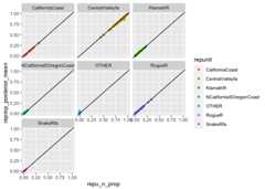
Quite often you might be curious about how much you can expect to beable to trust the posterior for individual fish from a mixture likethis. You can retrieve all the posteriors computed for the fishsimulated inassess_reference_loo() using thereturn_indiv_posteriors option. When you do this, thefunction returns a list with componentsmixture_proportions(which holds a tibble likechin_sims_repu_top6 in theprevious section) andindiv_posteriors, which holds all theposteriors (PofZs) for the simulated individuals.
set.seed(100)chin_sims_with_indivs<-assess_reference_loo(reference = chinook,gen_start_col =5,reps =50,mixsize =200,alpha_repunit = arep,return_indiv_posteriors =TRUE)#> Warning: `as.tibble()` is deprecated as of tibble 2.0.0.#> Please use `as_tibble()` instead.#> The signature and semantics have changed, see `?as_tibble`.#> This warning is displayed once every 8 hours.#> Call `lifecycle::last_warnings()` to see where this warning was generated.# print out the indiv posteriorschin_sims_with_indivs$indiv_posteriors#> # A tibble: 690,000 x 9#> repunit_scenario collection_scen… iter indiv simulated_repun…#> <chr> <chr> <int> <int> <chr>#> 1 1 1 1 1 CentralValleyfa#> 2 1 1 1 1 CentralValleyfa#> 3 1 1 1 1 CentralValleyfa#> 4 1 1 1 1 CentralValleyfa#> 5 1 1 1 1 CentralValleyfa#> 6 1 1 1 1 CentralValleyfa#> 7 1 1 1 1 CentralValleyfa#> 8 1 1 1 1 CentralValleyfa#> 9 1 1 1 1 CentralValleyfa#> 10 1 1 1 1 CentralValleyfa#> # … with 689,990 more rows, and 4 more variables: simulated_collection <chr>,#> # repunit <chr>, collection <chr>, PofZ <dbl>In this tibble: -indiv is an integer specifier of thesimulated individual -simulated_repunit is the reportingunit the individual was simulated from -simulated_collection is the collection the simulatedgenotype came from -PofZ is the mean over the MCMC of theposterior probability that the individual originated from thecollection.
Now that we have done that, we can see what the distribution ofposteriors to the correct reporting unit is for fish from the differentsimulated collections. We’ll do that with a boxplot, coloring byrepunit:
# summarise thingsrepu_pofzs<- chin_sims_with_indivs$indiv_posteriors%>%filter(repunit== simulated_repunit)%>%group_by(iter, indiv, simulated_collection, repunit)%>%# first aggregate over reporting unitssummarise(repu_PofZ =sum(PofZ))%>%ungroup()%>%arrange(repunit, simulated_collection)%>%mutate(simulated_collection =factor(simulated_collection,levels =unique(simulated_collection)))#> `summarise()` regrouping output by 'iter', 'indiv', 'simulated_collection' (override with `.groups` argument)# also get the number of simulated individuals from each collectionnum_simmed<- chin_sims_with_indivs$indiv_posteriors%>%group_by(iter, indiv)%>%slice(1)%>%ungroup()%>%count(simulated_collection)# note, the last few steps make simulated collection a factor so that collections within# the same repunit are grouped together in the plot.# now, plot itggplot(repu_pofzs,aes(x = simulated_collection,y = repu_PofZ))+geom_boxplot(aes(colour = repunit))+geom_text(data = num_simmed,mapping =aes(y =1.025,label = n),angle =90,hjust =0,vjust =0.5,size =3)+theme(axis.text.x =element_text(angle =90,hjust =1,size =9,vjust =0.5))+ylim(c(NA,1.05))
Great. That is helpful.
By default, individuals are simulated inassess_reference_loo() by resampling full multilocusgenotypes. This tends to be more realistic, because it includes asmissing in the simulations all the missing data for individuals in thereference. However, as all the genes in individuals that have beenincorrectly placed in a reference stay together, that individual mighthave a low value of PofZ to the population it was simulated from. Due tothe latter issue, it might also yield a more pessimistic assessment’ ofthe power for GSI.
An alternative is to resample over gene copies—the CV-GC method ofAnderson, Waples, and Kalinowski (2008).
Let us do that and see how the simulated PofZ results change. Here wedo the simulations…
set.seed(101)# for reproducibility# do the simulationchin_sims_by_gc<-assess_reference_loo(reference = chinook,gen_start_col =5,reps =50,mixsize =200,alpha_repunit = arep,return_indiv_posteriors =TRUE,resampling_unit ="gene_copies")and here we process the output and plot it:
# summarise thingsrepu_pofzs_gc<- chin_sims_by_gc$indiv_posteriors%>%filter(repunit== simulated_repunit)%>%group_by(iter, indiv, simulated_collection, repunit)%>%# first aggregate over reporting unitssummarise(repu_PofZ =sum(PofZ))%>%ungroup()%>%arrange(repunit, simulated_collection)%>%mutate(simulated_collection =factor(simulated_collection,levels =unique(simulated_collection)))#> `summarise()` regrouping output by 'iter', 'indiv', 'simulated_collection' (override with `.groups` argument)# also get the number of simulated individuals from each collectionnum_simmed_gc<- chin_sims_by_gc$indiv_posteriors%>%group_by(iter, indiv)%>%slice(1)%>%ungroup()%>%count(simulated_collection)# note, the last few steps make simulated collection a factor so that collections within# the same repunit are grouped together in the plot.# now, plot itggplot(repu_pofzs_gc,aes(x = simulated_collection,y = repu_PofZ))+geom_boxplot(aes(colour = repunit))+geom_text(data = num_simmed_gc,mapping =aes(y =1.025,label = n),angle =90,hjust =0,vjust =0.5,size =3)+theme(axis.text.x =element_text(angle =90,hjust =1,size =9,vjust =0.5))+ylim(c(NA,1.05))
And in that, we find somewhat fewer fish that have low posteriors,but there are still some. This reminds us that with this dataset,(rather) occasionally it is possible to get individuals carryinggenotypes that make it difficult to correctly assign them to reportingunit.
If you are simulating the reporting unit proportions or numbers, andwant to have more control over which collections those fish aresimulated from, within the reporting units, then thesub_ppn andsub_dirichlet settings are foryou. These are given as column names in thealpha_collection data frame.
For example, let’s say we want to simulate reporting unit proportionsas before, usingarep from above:
arep#> # A tibble: 6 x 2#> repunit dirichlet#> <chr> <dbl>#> 1 CentralValleyfa 8.19#> 2 KlamathR 0.675#> 3 RogueR 0.608#> 4 CaliforniaCoast 0.298#> 5 NCaliforniaSOregonCoast 0.0927#> 6 SnakeRfa 0.0320But, now, let’s say that within reporting unit we want specificweights for different collections. Then we could specify those, forexample, like this:
arep_subs<-tribble(~collection,~sub_ppn,"Eel_R",0.1,"Russian_R",0.9,"Butte_Cr_fa",0.7,"Feather_H_sp",0.3)Collections that are not listed are given equal proportionswithin repunits that had no collections listed. However, if acollection is not listed, but other collections within its repunit are,then its simulated proportion will be zero. (Technically, it is notzero, but it is so small—like (10^{-8}) that is is effectively 0…doingthat made coding it up a lot easier…)
Now, we can simulate with that and see what the resulting proportionof fish from each collection is:
chin_sims_sub_ppn<-assess_reference_loo(reference = chinook,gen_start_col =5,reps =50,mixsize =200,alpha_repunit = arep,alpha_collection = arep_subs,return_indiv_posteriors =FALSE)# don't bother returning individual posteriorsNow observe the average proportions of the collections and repunitsthat were simulated, and the average fraction,within reportingunits of each of the collection
chin_sims_sub_ppn%>%group_by(repunit, collection)%>%summarise(mean_pi =mean(true_pi))%>%group_by(repunit)%>%mutate(repunit_mean_pi =sum(mean_pi),fract_within = mean_pi/ repunit_mean_pi)%>%mutate(fract_within =ifelse(fract_within<1e-06,0, fract_within))%>%# anything less than 1 in a million gets called 0filter(repunit_mean_pi>0.0)#> `summarise()` regrouping output by 'repunit' (override with `.groups` argument)#> # A tibble: 17 x 5#> # Groups: repunit [6]#> repunit collection mean_pi repunit_mean_pi fract_within#> <chr> <chr> <dbl> <dbl> <dbl>#> 1 CaliforniaCoast Eel_R 3.57e-3 0.0357 0.1#> 2 CaliforniaCoast Russian_R 3.21e-2 0.0357 0.9#> 3 CentralValleyfa Battle_Cr 8.28e-8 0.828 0#> 4 CentralValleyfa Butte_Cr_fa 5.79e-1 0.828 0.700#> 5 CentralValleyfa Deer_Cr_fa 8.28e-8 0.828 0#> 6 CentralValleyfa Feather_H_fa 8.28e-8 0.828 0#> 7 CentralValleyfa Feather_H_sp 2.48e-1 0.828 0.300#> 8 CentralValleyfa Mill_Cr_fa 8.28e-8 0.828 0#> 9 CentralValleyfa Mokelumne_R_fa 8.28e-8 0.828 0#> 10 CentralValleyfa Sacramento_R_… 8.28e-8 0.828 0#> 11 KlamathR Klamath_IGH_fa 3.11e-2 0.0622 0.5#> 12 KlamathR Trinity_H_sp 3.11e-2 0.0622 0.5#> 13 NCaliforniaSOregonCo… Chetco_R 5.51e-3 0.0110 0.5#> 14 NCaliforniaSOregonCo… Smith_R 5.51e-3 0.0110 0.5#> 15 RogueR Applegate_Cr 2.69e-2 0.0539 0.5#> 16 RogueR Cole_Rivers_H 2.69e-2 0.0539 0.5#> 17 SnakeRfa Lyons_Ferry_H 9.61e-3 0.00961 1In the fisheries world, “100% simulations” have been a staple. Inthese simulations, mixtures are simulated in which 100% of theindividuals are from one collection (or reporting unit, I suppose). Erichas never been a big fan of these since they don’t necessarily tell youhow you might do inferring actual mixtures that you might encounter.Nonetheless, since they have been such a mainstay in the field, it isworthwile showing how to do 100% simulations usingrubias.Furthermore, when people asked for this feature it made it clear thatEric had to provide a way to simulate multiple different scenarioswithout re-processing the reference data set each time. So this is whatI came up with: the way we do it is to pass alist of scenariosto thealpha_repunit oralpha_collectionoption inassess_reference_loo(). These can be named lists,if desired. So, for example, let’s do 100% simulations for each of therepunits inarep:
arep$repunit#> [1] "CentralValleyfa" "KlamathR"#> [3] "RogueR" "CaliforniaCoast"#> [5] "NCaliforniaSOregonCoast" "SnakeRfa"We will let the collections within them just be drawn from adirichlet distribution with parameter 10 (so, pretty close to equalproportions).
So, to do this, we make a list of data frames with the proportions.We’ll give it some names too:
six_hundy_scenarios<-lapply(arep$repunit,function(x)tibble(repunit = x,ppn =1.0))names(six_hundy_scenarios)<-paste("All", arep$repunit,sep ="-")Then, we use it, producing only 5 replicates for each scenario:
repu_hundy_results<-assess_reference_loo(reference = chinook,gen_start_col =5,reps =5,mixsize =50,alpha_repunit = six_hundy_scenarios,alpha_collection =10)#> ++++ Starting in on repunit_scenario All-CentralValleyfa with collection scenario 1 ++++#> Doing LOO simulations rep 1 of 5#> Doing LOO simulations rep 2 of 5#> Doing LOO simulations rep 3 of 5#> Doing LOO simulations rep 4 of 5#> Doing LOO simulations rep 5 of 5#> ++++ Starting in on repunit_scenario All-KlamathR with collection scenario 1 ++++#> Doing LOO simulations rep 1 of 5#> Doing LOO simulations rep 2 of 5#> Doing LOO simulations rep 3 of 5#> Doing LOO simulations rep 4 of 5#> Doing LOO simulations rep 5 of 5#> ++++ Starting in on repunit_scenario All-RogueR with collection scenario 1 ++++#> Doing LOO simulations rep 1 of 5#> Doing LOO simulations rep 2 of 5#> Doing LOO simulations rep 3 of 5#> Doing LOO simulations rep 4 of 5#> Doing LOO simulations rep 5 of 5#> ++++ Starting in on repunit_scenario All-CaliforniaCoast with collection scenario 1 ++++#> Doing LOO simulations rep 1 of 5#> Doing LOO simulations rep 2 of 5#> Doing LOO simulations rep 3 of 5#> Doing LOO simulations rep 4 of 5#> Doing LOO simulations rep 5 of 5#> ++++ Starting in on repunit_scenario All-NCaliforniaSOregonCoast with collection scenario 1 ++++#> Doing LOO simulations rep 1 of 5#> Doing LOO simulations rep 2 of 5#> Doing LOO simulations rep 3 of 5#> Doing LOO simulations rep 4 of 5#> Doing LOO simulations rep 5 of 5#> ++++ Starting in on repunit_scenario All-SnakeRfa with collection scenario 1 ++++#> Doing LOO simulations rep 1 of 5#> Doing LOO simulations rep 2 of 5#> Doing LOO simulations rep 3 of 5#> Doing LOO simulations rep 4 of 5#> Doing LOO simulations rep 5 of 5repu_hundy_results#> # A tibble: 2,070 x 9#> repunit_scenario collection_scen… iter repunit collection true_pi n#> <chr> <chr> <int> <chr> <chr> <dbl> <dbl>#> 1 All-CentralVall… 1 1 Centra… Feather_H… 0.100 5#> 2 All-CentralVall… 1 1 Centra… Butte_Cr_… 0 0#> 3 All-CentralVall… 1 1 Centra… Mill_Cr_sp 0 0#> 4 All-CentralVall… 1 1 Centra… Deer_Cr_sp 0 0#> 5 All-CentralVall… 1 1 Centra… UpperSacr… 0 0#> 6 All-CentralVall… 1 1 Centra… Feather_H… 0.141 5#> 7 All-CentralVall… 1 1 Centra… Butte_Cr_… 0.100 5#> 8 All-CentralVall… 1 1 Centra… Mill_Cr_fa 0.140 5#> 9 All-CentralVall… 1 1 Centra… Deer_Cr_fa 0.193 14#> 10 All-CentralVall… 1 1 Centra… Mokelumne… 0.102 5#> # … with 2,060 more rows, and 2 more variables: post_mean_pi <dbl>,#> # mle_pi <dbl>Just to make sure that it is clear how to do this with collections(rather than reporting units) as well, lets do 100% simulations for ahandful of the collections. Let’s just randomly take 5 of them, and do 6reps for each:
set.seed(10)hundy_colls<-sample(unique(chinook$collection),5)hundy_colls#> [1] "Deer_Cr_fa" "Kitwanga_R" "Morice_R" "Wenatchee_R" "Russian_R"So, now make a list of those with 100% specifications in thetibbles:
hundy_coll_list<-lapply(hundy_colls,function(x)tibble(collection = x,ppn =1.0))%>%setNames(paste("100%", hundy_colls,sep ="_"))Then, do it:
hundy_coll_results<-assess_reference_loo(reference = chinook,gen_start_col =5,reps =6,mixsize =50,alpha_collection = hundy_coll_list)hundy_coll_results#> # A tibble: 2,070 x 9#> repunit_scenario collection_scen… iter repunit collection true_pi n#> <chr> <chr> <int> <chr> <chr> <dbl> <dbl>#> 1 1 100%_Deer_Cr_fa 1 Centra… Feather_H… 0 0#> 2 1 100%_Deer_Cr_fa 1 Centra… Butte_Cr_… 0 0#> 3 1 100%_Deer_Cr_fa 1 Centra… Mill_Cr_sp 0 0#> 4 1 100%_Deer_Cr_fa 1 Centra… Deer_Cr_sp 0 0#> 5 1 100%_Deer_Cr_fa 1 Centra… UpperSacr… 0 0#> 6 1 100%_Deer_Cr_fa 1 Centra… Feather_H… 0 0#> 7 1 100%_Deer_Cr_fa 1 Centra… Butte_Cr_… 0 0#> 8 1 100%_Deer_Cr_fa 1 Centra… Mill_Cr_fa 0 0#> 9 1 100%_Deer_Cr_fa 1 Centra… Deer_Cr_fa 1 50#> 10 1 100%_Deer_Cr_fa 1 Centra… Mokelumne… 0 0#> # … with 2,060 more rows, and 2 more variables: post_mean_pi <dbl>,#> # mle_pi <dbl>These are obtained usingmethod = "PB" ininfer_mixture(). When invoked, this will return the regularMCMC results as before, but also will population thebootstrapped_proportions field of the output. Doing sotakes a little bit longer, computationally, because there is a good dealof simulation involved:
mix_est_pb<-infer_mixture(reference = chinook,mixture = chinook_mix,gen_start_col =5,method ="PB")And now we can compare the estimates, showing here the 10 mostprevalent repunits, in therec1 fishery:
mix_est_pb$mixing_proportions%>%group_by(mixture_collection, repunit)%>%summarise(repprop =sum(pi))%>%left_join(mix_est_pb$bootstrapped_proportions)%>%ungroup()%>%filter(mixture_collection=="rec1")%>%arrange(desc(repprop))%>%slice(1:10)It gives us a result that we expect: no appreciable difference,because the reporting units are already very well resolved, so we don’texpect that the parametric bootstrap procedure would find any benefit incorrecting them.
Anderson, Eric C, Robin S Waples, and Steven T Kalinowski. 2008. “AnImproved Method for Predicting the Accuracy of Genetic StockIdentification.”Can J Fish Aquat Sci 65: 1475–86.