RStanKritian Brock
trialr is a collection of Bayesian clinical trialdesigns implemented in Stan and R. The documentation is available athttps://brockk.github.io/trialr/
There are many notable Bayesian designs and methods for clinicaltrials. However, one of the factors that has constrained their use isthe availability of software. We present here some of the most popular,implemented and demonstrated in a consistent style, leveraging thepowerful Stan environment for Bayesian computing.
Implementations exist in other R packages. Sometimes authors makeavailable code with their publications. However, challenges to use stillpersist. Different methods are presented in disparate styles. Featuresimplemented in one package for one design may be missing in another.Sometimes the technology chosen may only be available on a particularoperating system, or the chosen technology may have fallen intodisuse.
trialr seeks to address these problems. Models arespecified inStan, a state-of-the-artenvironment for Bayesian analysis. It uses Hamiltonian Monte Carlo totake samples from the posterior distribution. This method is moreefficient than Gibbs sampling and reliable inference can usually beperformed on a few thousand posterior samples. R, Stan andtrialr are each available on Mac, Linux, and Windows, soall of the examples presented here work on each operating system.Furthermore, Stan offers a very simple method to split the samplingacrossn cores, taking full advantage of the modern multicoreprocessors.
The designs implemented intrialr are introduced brieflybelow, and developed more fully in vignettes. We focus on real-lifeusage, including:
ggplotgraphics.In all examples, we will need to loadtrialr
library(trialr)The Continual Reassessment Method (CRM) was first published byO’Quigley, Pepe, and Fisher (1990). It assumes a smooth mathematicalform for the dose-toxicity curve to conduct a dose-finding trial seekinga maximum tolerable dose. There are many variations to suit differentclinical scenarios and the design has enjoyed relatively common use,although nowhere near as common as the ubiquitous and inferior 3+3design.
We will demonstrate the method using a notional trial example. In ascenario of five doses, we seek the dose with probability of toxicityclosest to 25% where our prior guesses of the rates of toxicity can berepresented:
target<-0.25skeleton<-c(0.05,0.15,0.25,0.4,0.6)Let us assume that we have already treated 2 patients each at doses2, 3 and 4, having seen two toxicities at dose-level 4 and noneelsewhere. What dose should we give to the next patient or cohort? Wefit the data to the popular empiric variant of the CRM model:
fit1<-stan_crm(outcome_str ='2NN 3NN 4TT',skeleton = skeleton,target = target,model ='empiric',beta_sd =sqrt(1.34),seed =123)The parameteroutcome_str = '2NN 3NN 4TT' reflects thattwo patients each have been treated at doses 2, 3, and 4, and that thetwo patients at dose 4 had toxicity but the other patients did not.
The fitted model contains lots of useful of information:
fit1#> Patient Dose Toxicity Weight#> 1 1 2 0 1#> 2 2 2 0 1#> 3 3 3 0 1#> 4 4 3 0 1#> 5 5 4 1 1#> 6 6 4 1 1#>#> Dose Skeleton N Tox ProbTox MedianProbTox ProbMTD#> 1 1 0.05 0 0 0.108 0.0726 0.2140#> 2 2 0.15 2 0 0.216 0.1900 0.2717#> 3 3 0.25 2 0 0.310 0.2972 0.2657#> 4 4 0.40 2 2 0.444 0.4484 0.2090#> 5 5 0.60 0 0 0.624 0.6395 0.0395#>#> The model targets a toxicity level of 0.25.#> The dose with estimated toxicity probability closest to target is 2.#> The dose most likely to be the MTD is 2.#> Model entropy: 1.49library(ggplot2)library(tidybayes)library(dplyr)fit1%>%spread_draws(prob_tox[Dose])%>%ggplot(aes(x = Dose,y = prob_tox))+stat_interval(.width =c(.5, .8, .95))+scale_color_brewer()+labs(y ='Prob(DLT)',title ='Posterior dose-toxicity beliefs using empiric CRM')
Several variants of the CRM are implemented in ‘trialr’. These aredemonstrated in the CRM vignette. Several visualisation techniques areillustrated in theVisualisation in CRM vignette. Thetime-to-event CRM is introduced in the TITE-CRM vignette.
Neuenschwander, Branson, and Gsponer (2008) introduced atwo-parameter logistic model for dose-escalation. It shares manycharacteristics of the CRM models presented above but instead of askeleton, it uses as a covariate the doses under investigation dividedby some reference dose.
E.g., reproducing one of the analyses in their paper:
dose<-c(1,2.5,5,10,15,20,25,30,40,50,75,100,150,200,250)d_star<-250target<-0.30outcomes<-'1NNN 2NNNN 3NNNN 4NNNN 7TT'fit<-stan_nbg(outcome_str = outcomes,real_doses = dose,d_star = d_star,target = target,alpha_mean =2.15,alpha_sd =0.84,beta_mean =0.52,beta_sd =0.8,seed =2020,refresh =0)fit#> Patient Dose Toxicity Weight#> 1 1 1 0 1#> 2 2 1 0 1#> 3 3 1 0 1#> 4 4 2 0 1#> 5 5 2 0 1#> 6 6 2 0 1#> 7 7 2 0 1#> 8 8 3 0 1#> 9 9 3 0 1#> 10 10 3 0 1#> 11 11 3 0 1#> 12 12 4 0 1#> 13 13 4 0 1#> 14 14 4 0 1#> 15 15 4 0 1#> 16 16 7 1 1#> 17 17 7 1 1#>#> Dose N Tox ProbTox MedianProbTox ProbMTD#> 1 1 3 0 0.0126 0.00563 0.00025#> 2 2 4 0 0.0325 0.01967 0.00050#> 3 3 4 0 0.0675 0.04934 0.02250#> 4 4 4 0 0.1385 0.11863 0.10450#> 5 5 0 0 0.2064 0.18937 0.16775#> 6 6 0 0 0.2692 0.25641 0.17100#> 7 7 2 2 0.3264 0.31878 0.14425#> 8 8 0 0 0.3780 0.37409 0.16850#> 9 9 0 0 0.4661 0.46884 0.12475#> 10 10 0 0 0.5371 0.54698 0.07125#> 11 11 0 0 0.6616 0.67700 0.02000#> 12 12 0 0 0.7390 0.75753 0.00375#> 13 13 0 0 0.8259 0.84691 0.00075#> 14 14 0 0 0.8717 0.89297 0.00025#> 15 15 0 0 0.8993 0.91986 0.00000#>#> The model targets a toxicity level of 0.3.#> The dose with estimated toxicity probability closest to target is 7.#> The dose most likely to be the MTD is 6.#> Model entropy: 2.06This reproduces the inferences depicted in the lower right pane ofFigure 1 in Neuenschwander, Branson, and Gsponer (2008).
For more, see theTwo-parameter logistic model for dose-findingby Neuenschwander, Branson & Gsponer vignette.
EffTox by Thall and Cook (2004) is a dose-finding design that usesbinary efficacy and toxicity outcomes to select a dose with a highutility score. We present it briefly here but there is a much morethorough examination in the EffTox vignette.
For demonstration, we fit the model parameterisation introduced byThall et al. (2014) to the following notional outcomes:
| Patient | Dose-level | Toxicity | Efficacy |
|---|---|---|---|
| 1 | 1 | 0 | 0 |
| 2 | 1 | 0 | 0 |
| 3 | 1 | 0 | 1 |
| 4 | 2 | 0 | 1 |
| 5 | 2 | 0 | 1 |
| 6 | 2 | 1 | 1 |
outcomes<-'1NNE 2EEB'fit2<-stan_efftox_demo(outcomes,seed =123)In an efficacy and toxicity dose-finding scenario, the number ofpatient outcomes has increased. It is possible that patients experienceefficacy only (E), toxicity only (T), both (B) or neither (N).
fit2#> Patient Dose Toxicity Efficacy#> 1 1 1 0 0#> 2 2 1 0 0#> 3 3 1 0 1#> 4 4 2 0 1#> 5 5 2 0 1#> 6 6 2 1 1#>#> Dose N ProbEff ProbTox ProbAccEff ProbAccTox Utility Acceptable ProbOBD#> 1 1 3 0.402 0.088 0.333 0.927 -0.342 TRUE 0.0465#> 2 2 3 0.789 0.103 0.943 0.921 0.412 TRUE 0.2625#> 3 3 0 0.929 0.225 0.984 0.718 0.506 TRUE 0.2077#> 4 4 0 0.955 0.315 0.983 0.617 0.420 FALSE 0.0620#> 5 5 0 0.964 0.372 0.980 0.561 0.349 FALSE 0.4213#>#> The model recommends selecting dose-level 3.#> The dose most likely to be the OBD is 5.#> Model entropy: 1.36In this example, after evaluation of our six patients, the doseadvocated for the next group is dose-level 3. This is contained in thefitted object:
fit2$recommended_dose#> [1] 3This is not surprising because dose 3 has the highest utilityscore:
fit2$utility#> [1] -0.3418428 0.4120858 0.5064312 0.4199298 0.3493254Sometimes, doses other than the maximal-utility dose will berecommended because of the dose-admissibility rules. See the EffToxvignette and the original papers for more details.
Functions are provided to create useful plots. For instance, it isilluminating to plot the posterior means of the probabilities ofefficacy and toxicity at each of the doses on the trade-off contoursused to measure dose attractiveness. The five doses are shown in red.Doses closer to the lower-right corner have higher utility.
efftox_contour_plot(fit2)title('EffTox utility contours')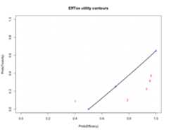
This example continues in the EffTox vignette. There are manypublications related to EffTox, including Thall and Cook (2004) andThall et al. (2014).
Sticking with Peter Thall’s huge contribution to Bayesian clinicaltrials, Thall et al. (2003) described a method for analysing treatmenteffects of a single intervention in several sub-types of a singledisease.
We demonstrate the method for partially-pooling response rates to asingle drug in various subtypes of sarcoma. This example is used inThall et al. (2003). Fitting the data to the model:
fit3<-stan_hierarchical_response_thall(group_responses =c(0,0,1,3,5,0,1,2,0,0),group_sizes =c(0,2 ,1,7,5,0,2,3,1,0),mu_mean =-1.3863,mu_sd =sqrt(1/0.1),tau_alpha =2,tau_beta =20)mu andtau are mean and precisionparameters for the partially-pooled effects in the model.mu_mean andmu_sd are hyperparameters for anormal prior, andtau_alpha andtau_beta arehyperparameters for an inverse gamma prior. This specification isdescribed in the original model.
The returned object is the same type as the fits returned byrstan:
fit3#> Inference for Stan model: ThallHierarchicalBinary.#> 4 chains, each with iter=2000; warmup=1000; thin=1;#> post-warmup draws per chain=1000, total post-warmup draws=4000.#>#> mean se_mean sd 2.5% 25% 50% 75% 97.5% n_eff#> mu -0.04 0.03 1.38 -2.86 -0.89 -0.02 0.86 2.60 2295#> sigma2 13.22 0.59 16.18 3.45 6.44 9.56 14.77 43.41 748#> rho[1] -0.03 0.07 3.87 -8.25 -2.26 0.08 2.29 7.20 3079#> rho[2] -3.03 0.06 2.63 -9.68 -4.20 -2.55 -1.31 0.69 1899#> rho[3] 2.46 0.07 2.86 -1.87 0.65 2.06 3.83 9.13 1497#> rho[4] -0.31 0.01 0.79 -1.87 -0.82 -0.31 0.21 1.22 4031#> rho[5] 3.76 0.06 2.42 0.59 2.11 3.31 4.78 10.04 1448#> rho[6] -0.09 0.07 3.85 -8.34 -2.27 0.02 2.27 7.41 3092#> rho[7] 0.06 0.03 1.53 -2.90 -0.92 0.09 0.99 3.05 3658#> rho[8] 0.75 0.02 1.31 -1.55 -0.12 0.65 1.52 3.65 2785#> rho[9] -2.43 0.07 2.91 -9.18 -3.86 -2.00 -0.50 2.09 1919#> rho[10] 0.01 0.07 3.97 -7.85 -2.29 0.05 2.38 7.74 2982#> sigma 3.38 0.05 1.33 1.86 2.54 3.09 3.84 6.59 819#> prob_response[1] 0.50 0.01 0.38 0.00 0.09 0.52 0.91 1.00 3476#> prob_response[2] 0.15 0.00 0.18 0.00 0.01 0.07 0.21 0.67 3817#> prob_response[3] 0.78 0.00 0.25 0.13 0.66 0.89 0.98 1.00 4141#> prob_response[4] 0.43 0.00 0.17 0.13 0.31 0.42 0.55 0.77 4036#> prob_response[5] 0.92 0.00 0.10 0.64 0.89 0.96 0.99 1.00 3879#> prob_response[6] 0.50 0.01 0.38 0.00 0.09 0.51 0.91 1.00 3564#> prob_response[7] 0.51 0.00 0.27 0.05 0.28 0.52 0.73 0.95 3642#> prob_response[8] 0.64 0.00 0.22 0.18 0.47 0.66 0.82 0.97 3040#> prob_response[9] 0.23 0.00 0.26 0.00 0.02 0.12 0.38 0.89 3971#> prob_response[10] 0.50 0.01 0.38 0.00 0.09 0.51 0.92 1.00 2970#> lp__ -34.42 0.15 3.77 -43.20 -36.48 -33.86 -31.71 -28.88 611#> Rhat#> mu 1#> sigma2 1#> rho[1] 1#> rho[2] 1#> rho[3] 1#> rho[4] 1#> rho[5] 1#> rho[6] 1#> rho[7] 1#> rho[8] 1#> rho[9] 1#> rho[10] 1#> sigma 1#> prob_response[1] 1#> prob_response[2] 1#> prob_response[3] 1#> prob_response[4] 1#> prob_response[5] 1#> prob_response[6] 1#> prob_response[7] 1#> prob_response[8] 1#> prob_response[9] 1#> prob_response[10] 1#> lp__ 1#>#> Samples were drawn using NUTS(diag_e) at Thu Oct 15 09:52:56 2020.#> For each parameter, n_eff is a crude measure of effective sample size,#> and Rhat is the potential scale reduction factor on split chains (at#> convergence, Rhat=1).So, we can use the underlying plot method inrstan.
library(rstan)library(ggplot2)plot(fit3,pars ='prob_response')+geom_vline(xintercept =0.3,col ='orange',linetype ='dashed')+labs(title ='Partially-pooled response rates in 10 sarcoma subtypes')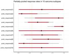
The hierarchical model for binary responses is developed in its ownvignette.
Thall, Nguyen, and Estey (2008) introduced an extension of EffToxthat allows dose-finding by efficacy and toxicity outcomes and adjustsfor covariate information. Brock, et al. (manuscript accepted but notyet in press) simplified the method by removing the dose-findingcomponents to leave a design that studies associated co-primary andtoxicity outcomes in an arbitrary number of cohorts determined by thebasline covariates. They refered to the simplifed design as BEBOP, forBayesian Evaluation of Bivariate binary Outcomes with Predictivevariables.
The investigators implement the design is a phase II trial ofpembrolizumab in non-small-cell lung cancer. A distinct feature of thetrial is the availability of predictive baseline covariates, the mostnoteworthy of which is the PD-L1 tumour proportion score, shown by Garonet al. (2015) to be a predictive biomarker for drug efficacy.
This example is demonstrated in the BEBOP vignette.
You can install the latest trialr commit from github with:
# install.packages("devtools")devtools::install_github("brockk/trialr")You can install the latest CRAN release by running:
install.packages("trialr")It should go without saying that the CRAN release will be older thanthe github version.
If there is a published Bayesian design you want implemented in Stan,get in touch. Contact brockk on github.
Garon, Edward B, Naiyer a Rizvi, Rina Hui, Natasha Leighl, Ani SBalmanoukian, Joseph Paul Eder, Amita Patnaik, et al. 2015.“Pembrolizumab for the Treatment of Non-Small-Cell Lung Cancer.”TheNew England Journal of Medicine 372 (21): 2018–28.https://doi.org/10.1056/NEJMoa1501824.
Neuenschwander, Beat, Michael Branson, and Thomas Gsponer. 2008.“Critical Aspects of the Bayesian Approach to Phase I Cancer Trials.”Statistics in Medicine 27 (13): 2420–39.https://doi.org/10.1002/sim.3230.
O’Quigley, J, M Pepe, and L Fisher. 1990. “Continual ReassessmentMethod: A Practical Design for Phase 1 Clinical Trials in Cancer.”Biometrics 46 (1): 33–48.https://doi.org/10.2307/2531628.
Thall, Peter F., Hoang Q. Nguyen, and Elihu H. Estey. 2008.“Patient-Specific Dose Finding Based on Bivariate Outcomes andCovariates.”Biometrics 64 (4): 1126–36.https://doi.org/10.1111/j.1541-0420.2008.01009.x.
Thall, Peter F., J. Kyle Wathen, B. Nebiyou Bekele, Richard E.Champlin, Laurence H. Baker, and Robert S. Benjamin. 2003. “HierarchicalBayesian Approaches to Phase II Trials in Diseases with MultipleSubtypes.”Statistics in Medicine 22 (5): 763–80.https://doi.org/10.1002/sim.1399.
Thall, PF, and JD Cook. 2004. “Dose-Finding Based onEfficacy-Toxicity Trade-Offs.”Biometrics 60 (3): 684–93.
Thall, PF, RC Herrick, HQ Nguyen, JJ Venier, and JC Norris. 2014.“Effective Sample Size for Computing Prior Hyperparameters in BayesianPhase I-II Dose-Finding.”Clinical Trials 11 (6): 657–66.https://doi.org/10.1177/1740774514547397.